library(tidyverse)Introduction
Experiments continue to grow in political science (Druckman and Green 2021), and designing an experiment requires us to either select an appropriate sample size or evaluate whether a given sample size is sufficient for our goals.For example, the Journal of Politics guidelines for registered reports note that “a detailed justification of the proposed sample size is crucial” (accessed October 20, 2026; persistent link). The Journal of Experimental Political Science requires authors to “explain how the sample size was determined and note statistical power” (accessed October 20, 2026; persistent link). Time-sharing Experiments for the Social Sciences (TESS) notes that power analysis is “encouraged” (accessed October 20, 2026; persistent link). The National Institutes of Health (NIH) provides several examples to “demonstrate rigor,” and all examples include a discussion of statistical power (accessed October 20, 2026; persistent link). The popular OSF pre-registration template includes a field for a sample size rationale, which could include a power analysis (Bowman et al. 2020). Statistical power, or the chance of rejecting the null hypothesis for a given treatment effect, is a common, powerful way to select or evaluate a sample size. The consequences of low power are increasingly understood: low power can lead to wildly overestimated treatment effects (Gelman and Carlin 2014) and ambiguous results that are difficult to publish (e.g., Alrababa’h et al. 2023). Nonetheless, Arel-Bundock et al. (2026) argue that only about 10% of statistical tests in political science have at least 80% power to detect the consensus effect in their literature. Stommes, Aronow, and Sävje (2023) find that regression discontinuity studies in political science tend to be underpowered as well. And political science is hardly unusual (Cohen 1962; Button et al. 2013; Ioannidis, Stanley, and Doucouliagos 2017; Stanley, Carter, and Doucouliagos 2018; Yang et al. 2023). Underscoring their important findings, Arel-Bundock et al. (2026, 44–45) emphasize: “our research community must address the problems of low power and selection on significance with institutional, methodological, and theoretical remedies.”
One apparent problem is that while political scientists understand estimation and inference for experimental data very well (e.g., least squares regression with robust standard errors), political scientists are less comfortable thinking about statistical power prior to data collection. This apparent discomfort is not without reason. Power analysis requires specialized software or tedious simulation. Most specialized software, such as G*Power (Faul et al. 2007; Faul et al. 2009), follows the conventions of psychology. The language (e.g., Cohen’s d) and style of analysis (e.g., ANCOVA) can make the software awkward for political scientists to use, though these obstacles are of course not insurmountable.For example, the power resources that the Journal of Politics provides include links to several resources for planning sample size in experiments, but many of these resources are directed primarily at psychologists. Most importantly, political scientists tend to focus on treatment effects on the scale of the outcome (e.g., King, Tomz, and Wittenberg 2000), while psychologists are more comfortable with standardized effect sizes.Lakens (2022) offers a careful and thorough discussion of sample size justifications for an audience of psychologists, but (appropriately) uses terms common in psychology. For example, Lakens centers much of his discussion around Cohen’s d, a standardized effect size used often in psychology but less often in political science. And while psychologists rely on a range of procedures to test hypotheses, political scientists typically use least squares regression with robust standard errors. In political science, recent conceptual work and statistical software (Blair et al. 2019; Blair, Coppock, and Humphreys 2023) make complex simulations to comprehensively evaluate research designs more accessible, but simulation to obtain statistical power remains challenging compared to analyzing experimental data. Political scientists lack a gateway between the simple, robust tools of inference using experimental data and the complex, tedious tools that allow complete and careful evaluations of research designs. This paper can help create the link by offering useful approximations for balanced, between-subjects designs or by helping build intuition that transfers to more complex designs.
In this paper, I offer several simple rules for assessing the statistical power of a balanced, between-subjects design (i.e., a design that assigns an equal number of subjects to each experimental condition). For these balanced, between-subjects designs (e.g., common for survey experiments), the rules are sufficient to demonstrate adequate power for treatment effects and interactions. I tightly connect the rules for statistical power to the logic of estimation and inference for experimental data in political science (least squares regression, robust standard errors, and confidence intervals). There is tremendous value in simple, conceptual rules of thumb—the kind of rules that allow us to predict the statistical power of an experiment with paper, a pencil, and (perhaps) a pocket calculator. While specialized software and complex simulations are helpful (and essential in some cases), simple rules have several benefits: (1) simple rules can make statistical power accessible, rather than seem like a mystical quantity; (2) simple rules allow us to reason fluently about design choices; (3) simple rules can reduce the chance of making big errors by giving us a ballpark starting point even if we ultimately rely on a more sophisticated approach; and (4) for balanced, between-subjects designs, simple rules are sufficient to justify a sample size, and simulations and specialized software are unnecessary. I explain the intuition of each rule, describe how we can use the rule to plan or evaluate a study, and give examples. Appendix 4 collects all seven rules in one place for quick reference.
Before turning to the rules, I should clearly delineate the type of experiments they cover, so that a reader can gauge whether the rules apply to their design. The rules in the main text apply to balanced (i.e., treatment and control groups are the same size), between-subjects experiments with independent assignment. I assume that we estimate the treatment effect with least squares regression and robust standard errors, and that we test a directional hypothesis about that effect. A researcher whose experiment fits this description can apply the rules in the main text directly.This includes experiments that analyze a multi-item index rather than a single item. A researcher analyzing an index can treat the index itself as the outcome (e.g., let \(\widetilde{SD(Y)}\) in Rule 3 be the standard deviation of the index rather than of a single item) and then proceed through the remaining rules as usual. For researchers whose experiment does not fit this description, we can accommodate several common complications discussed in Appendices 1 and 2. Appendix 1 gives the factors for power levels other than 80% or 95% for both the one-sided and two-sided conventions. Appendix 2 adapts the rules to unbalanced assignment, clustered assignment, blocked random assignment, and interactions. For designs with other complications, the rules might still provide a ballpark starting point, but a careful power analysis requires simulation or specialized software.
Review: The Estimation and Inference Framework
Throughout this discussion, I assume that we use ordinary least squares and robust standard errors to estimate the treatment effect. I assume size-0.05, one-sided tests of directional hypotheses (i.e., tests at the 0.05 significance level, or \(\alpha = 0.05\)) evaluated in practice using 90% confidence intervals. The one-sided test is a natural default because we test a directional hypothesis. Some researchers instead prefer two-sided tests, which are equivalent to 95% confidence intervals. I report the factors for two-sided tests alongside the one-sided factors throughout, so that researchers can apply the rules under either convention. To make the discussion more natural, I borrow the language of survey experiments and describe the experimental units as “respondents,” but the logic generalizes to other types of units (e.g., villages).
Formally, I assume potential outcomes \(\mathcal{Y}_{i}(1)\) if assigned to treatment and \(\mathcal{Y}_{i}(0)\) if assigned to control for respondent \(i\) of \(N\). An experiment might use more than two conditions, but for the sake of the discussion below, I focus on the statistical power of a comparison of just two of these conditions, which I call treatment and control.In many experiments, there will be multiple comparisons of interest. In this case, we need to compute the statistical power for each test separately. As the Journal of Politics guidelines note: “Power calculations should be performed for each test individually” (accessed October 20, 2026; persistent link). For these two conditions, we want to make inferences about the average treatment effect \(\tau = \frac{1}{N}\sum_{i = 1}^{N}{\mathcal{Y}_{i}(1)} - \frac{1}{N}\sum_{i = 1}^{N}{\mathcal{Y}_{i}(0)}\) (which I refer to as a “treatment effect” throughout).
To make inferences about \(\tau\), we randomly assign \(n_{1}\) respondents to treatment and \(n_{0}\) respondents to control, where \(N = n_{1} + n_{0}\).Note that \(N\) represents the total number of respondents in the comparison, while \(n_{d}\) represents the number of respondents in condition \(d \in \{0, 1\}\). Below, I assume equal numbers of respondents in each condition, so I let \(n\) represent the number of respondents per condition, which is a convenient quantity when thinking about experimental design and statistical power. We create an indicator variable \(D_{i}\) that equals 1 if the respondent is assigned to treatment and 0 if the respondent is assigned to control. Then we create the observed outcome \(Y_{i} = \mathcal{Y}_{i}\left( D_{i} \right)\) by assigning \(Y_{i}\) the potential outcome under treatment if \(D_{i} = 1\) and the potential outcome under control if \(D_{i} = 0\). Then we estimate the treatment effect using \(\widehat{\tau} = \frac{1}{n_{1}}\sum_{i = 1}^{N}{D_{i} \cdot Y_{i}} - \frac{1}{n_{0}}\sum_{i = 1}^{N}{\left( 1 - D_{i} \right) \cdot Y_{i}}\), which we compute in practice using least squares estimates of the model \(Y_{i} = \alpha + \tau \cdot D_{i} + \epsilon_{i}\). In some cases, we might increase the precision of the estimates by including variables measured pre-treatment as control variables in the regression model.
To estimate the standard error of \(\widehat{\tau}\), we use Neyman’s ([1923] 1990) conservative variance estimator.Specifically, \(\widehat{Var}\left( \widehat{\tau} \right) = \frac{s_{1}^{2}}{n_{1}} + \frac{s_{0}^{2}}{n_{0}}\), where \(s_{1}^{2}\) and \(s_{0}^{2}\) represent the sample variances in the treatment and control groups, respectively, and \({\widehat{SE}}_{\widehat{\tau}} = \sqrt{\widehat{Var}\left( \widehat{\tau} \right)}\). In practice, we use an HC2 heteroskedasticity-robust variance estimator (or a closely related variant).Samii and Aronow (2012, 367–368) show that the HC2 estimator is equivalent to Neyman’s estimator. For testing, Li and Ding (2017, 1764–1765) provide several additional (seemingly innocuous) regularity conditions such that a finite-population central limit theorem holds and \(\left\lbrack \widehat{\tau} - \Phi_{std}^{-1}\left( 1 - \alpha \right) \cdot {\widehat{SE}}_{\widehat{\tau}},\widehat{\tau} + \Phi_{std}^{-1}\left( 1 - \alpha \right) \cdot {\widehat{SE}}_{\widehat{\tau}} \right\rbrack\) is an asymptotically conservative \(\left( 1 - 2\alpha \right) \cdot 100\%\) confidence interval, where \(\Phi_{std}^{-1}\) is the inverse of the standard normal CDF. We can use the 90% confidence interval \(\left\lbrack \widehat{\tau} - 1.64 \cdot {\widehat{SE}}_{\widehat{\tau}},\widehat{\tau} + 1.64 \cdot {\widehat{SE}}_{\widehat{\tau}} \right\rbrack\) to conduct size-0.05 tests of directional hypotheses by rejecting a null hypothesis if and only if all values in the 90% confidence interval are consistent with the research hypothesis (Rainey 2014; McCaskey and Rainey 2015). A researcher using a size-0.05, two-sided test instead rejects the null hypothesis when the 95% confidence interval excludes zero. For the 95% confidence interval, the 1.64 threshold becomes 1.96 so that the 95% confidence interval is \(\left\lbrack \widehat{\tau} - 1.96 \cdot {\widehat{SE}}_{\widehat{\tau}},\widehat{\tau} + 1.96 \cdot {\widehat{SE}}_{\widehat{\tau}} \right\rbrack\).
Rules 1 and 2: What Is Statistical Power?
In a designed experiment, we usually have a theoretically motivated research hypothesis that we would like to test. This research hypothesis implies a null hypothesis that we hope to reject. For simplicity, I assume throughout much of this paper that we hypothesize a positive treatment effect so that \(H_{R}:\tau > 0\). The extension to a negative treatment effect is obvious.
Imagine that we repeatedly re-randomize to treatment and control and compute \(\widehat{\tau}\) for each repetition. Then \(\widehat{\tau}\) will vary across these repeated experiments. We refer to the distribution of \(\widehat{\tau}\) across these hypothetical repeated experiments as the sampling distribution of \(\widehat{\tau}\). This sampling distribution is typically centered over the treatment effect (i.e., \(\widehat{\tau}\) is unbiased or nearly so). Importantly, the standard deviation of the sampling distribution of \(\widehat{\tau}\) is called the standard error, and \({\widehat{SE}}_{\widehat{\tau}}\) is usually a precise estimator of the standard error.
If the research hypothesis \(H_{R}:\tau > 0\) is correct, then the sampling distribution of \(\widehat{\tau}\) lies mostly to the right of zero. However, we will only claim that \(\tau > 0\) if the entire 90% confidence interval is larger than zero, or, equivalently, if \(\widehat{\tau} - 1.64 \cdot {\widehat{SE}}_{\widehat{\tau}} > 0\). This means that we must design our experiment so that the sampling distribution falls relatively far from zero.
We say that the statistical power of an experiment is the chance of rejecting the null hypothesis for a particular treatment effect \(\tau\). For example, we say that an experiment has “80% power to detect a treatment effect of ” if \(\widehat{\tau} - 1.64 \cdot {\widehat{SE}}_{\widehat{\tau}} > 0\) in 80% of repeated experiments. Similarly, we say that the experiment has “95% power to detect a treatment effect of ” if \(\widehat{\tau} - 1.64 \cdot {\widehat{SE}}_{\widehat{\tau}} > 0\) in 95% of repeated experiments. By convention, 80% power is the minimal standard for “adequate” statistical power (Cohen 1988, 56), but others recommend higher power, such as 95%.For example, the Journal of Politics recommends “a power of at least 0.90, ideally 0.95, to detect anticipated/relevant effect sizes” for registered reports (accessed October 20, 2026; persistent link). Nature Human Behaviour requires that “the a priori power must be 0.95 or higher for all proposed hypothesis tests” for registered reports (accessed October 20, 2026; persistent link).
It turns out that statistical power is determined by the treatment effect and the standard error of the estimate. To compute the statistical power of an experiment, we must make assumptions or “informed guesses” about certain quantities. I denote these assumed values with a tilde. For example, I denote the assumed treatment effect as \(\widetilde{\tau}\).I use three different \(\tau\)s: the actual treatment effect \(\tau\), the treatment effect assumed for the sake of computing power \(\widetilde{\tau}\), and the estimated treatment effect \(\widehat{\tau}\). I read the tilde notation as “assumed to compute power.” For example, I read \(\widetilde{\tau}\) as “the treatment effect assumed to compute power.” The tilde notation also means “Wait! Think about this carefully; it is an assumption requiring judgment.” This just means “the treatment effect we are assuming for the sake of computing statistical power.”
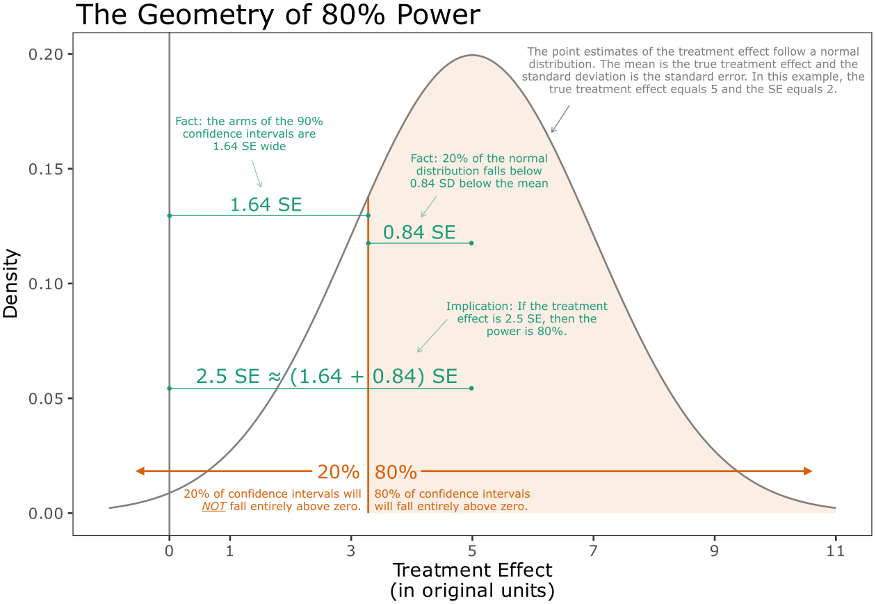
How can we compute the statistical power of an experiment? An intuitive approach uses the construction of the 90% confidence interval. Recall that we will reject the null hypothesis if the lower bound of the 90% confidence interval falls above zero. The arms of the 90% confidence interval are about 1.64 standard errors wide.I write “about” 1.64 standard errors because in practice we use the estimated standard error, not the actual standard error. However, the estimated standard error is sufficiently precise to treat the two interchangeably in this context. This means that we will reject the null hypothesis if the estimate of the treatment effect is larger than 1.64 standard errors. Thus, the power of the study is the percent of the sampling distribution that is larger than 1.64 standard errors. Recall that the sampling distribution is approximately normally distributed and centered over the treatment effect \(\tau\) with standard deviation equal to the standard error of the estimate of \(\tau\).Rule 1 is exact when (a) \(\widehat{\tau}\) is exactly normally distributed with mean \(\tau\) and standard deviation \(SE\) and (b) \(SE\) is known rather than estimated. Condition (a) holds in finite samples when errors are exactly normally distributed. It also holds asymptotically by the central limit theorem (CLT) under Li and Ding’s (2017) finite-population regularity conditions. Condition (b) is only approximate because the rejection rule uses \(\widehat{SE}\) and not the actual \(SE\). But for balanced, between-subjects designs with constant treatment effects, the Neyman (or HC2) estimator is consistent for the true sampling SE. (The error in this approximate statistical power is less than one percentage point at \(\tau/SE = 2.5\) and \(n = 50\) per condition.) Under the rules’ scope conditions (balanced, between-subjects experiments with independent assignment) and with sufficient \(n\) for the CLT, Rule 1 offers an excellent approximation. Thus, computing the power is simply computing the percent of the sampling distribution above \(1.64 \cdot SE\).
R code
# footnote 12: Rule 1 compared to simulated experiments that use the estimated SE
#   (balanced design, normal outcomes, constant treatment effect)
set.seed(1234)

# design
n     <- 50                # respondents per condition
sigma <- 1                 # SD of the outcome within each condition
se    <- 2*sigma/sqrt(2*n) # true SE (Rule 3)
tau   <- 2.5*se            # treatment effect, so that tau/SE = 2.5

# simulate experiments; reject if the lower bound of the 90% CI is above zero
#   - for a difference in means, the HC2 SE is sqrt(s1^2/n + s0^2/n)
simulate_experiments <- function(n_exp) {
  y0 <- matrix(rnorm(n_exp*n, mean = 0,   sd = sigma), nrow = n_exp)
  y1 <- matrix(rnorm(n_exp*n, mean = tau, sd = sigma), nrow = n_exp)
  row_var <- function(y) rowSums((y - rowMeans(y))^2)/(n - 1)
  tau_hat <- rowMeans(y1) - rowMeans(y0)
  se_hat  <- sqrt(row_var(y1)/n + row_var(y0)/n)
  tau_hat - 1.64*se_hat > 0
}
reject <- map(rep(10000, 100), simulate_experiments) %>% unlist()  # 1,000,000 experiments

# power from Rule 1 and simulated power
power_rule_1 <- 1 - pnorm(1.64*se, mean = tau, sd = se)
power_sim    <- mean(reject)
c(rule_1 = power_rule_1, simulation = power_sim)
rule_1 simulation
0.8051055 0.8046190 # difference (percentage points)
100*abs(power_sim - power_rule_1)[1] 0.04864787Rule 1 (Power; Most Intuitively): Power equals \(1 - \Phi(1.64 \cdot SE;\mu = \tau,\sigma = SE)\), where \(\Phi(z;\mu,\sigma)\) is the normal CDF, \(SE\) is the standard error of the estimated treatment effect, and \(\tau\) is the treatment effect.
See Gerber and Green (2012, 93) for a similar presentation.
Dividing through by the standard error and then subtracting \(\frac{\tau}{SE}\), we see that power also equals \(1 - \Phi\left( 1.64 - \frac{\tau}{SE};\mu = 0,\sigma = 1 \right)\); the values of \(\Phi\left(z;\mu = 0,\sigma = 1 \right)\) are provided in common \(z\) tables, where \(z = 1.64 - \frac{\tau}{SE}\). This allows us to compute power using the standard normal CDF.
Rule 2 (Power; From a \(z\) Table): Power equals \(1 - \Phi_{std}\left( 1.64 - \frac{\tau}{SE} \right)\), where \(\Phi_{std}(z)\) is the standard normal CDF (as found in a standard \(z\) table), \(SE\) is the standard error of the estimated treatment effect, and \(\tau\) is the treatment effect.
Rule 2 allows us to connect statistical power to the familiar \(z\) table in the appendices of many statistics textbooks or the pnorm() function in R. But, more importantly, it drives home a central intuition: power is determined by the key ratio \(\frac{\tau}{SE}\). To estimate power, we must make an informed assumption about the effect of interest and a good prediction of the standard error of the estimate. Further, when we consider changes to the experimental design and the consequences for statistical power, it can be helpful to think about the numerator or the denominator of the key ratio \(\frac{\tau}{SE}\): How do we make the effect as large as possible? And how do we make the estimate as precise as possible?
R code
# power for a treatment effect of 5 and a standard error of 2 (the case in Figure 1)
tau <- 5
se  <- 2

# Rule 1: the normal CDF with mean tau and standard deviation SE
1 - pnorm(1.64*se, mean = tau, sd = se)
[1] 0.8051055# Rule 2: the standard normal CDF (the same number)
1 - pnorm(1.64 - tau/se)[1] 0.8051055Check by simulation
# simulate the case in Figure 1: a treatment effect of 5 and a standard error of 2; any design
#   with that standard error will do, here 50 respondents per condition and outcomes with an SD
#   of 10 within each condition (Rule 3); analyze each experiment as in the paper (OLS with HC2
#   standard errors; reject if the lower bound of the 90% confidence interval is above zero)

library(sandwich)  # robust standard errors
library(lmtest)    # confidence intervals with robust standard errors

set.seed(1234)
n    <- 50
sd_y <- 10
tau  <- 5

simulate_experiment <- function() {
  y0  <- rnorm(2*n, mean = 0, sd = sd_y)   # potential outcomes under control...
  y1  <- y0 + tau                          # ...and under treatment
  z   <- sample(rep(0:1, each = n))        # n respondents to each condition, at random
  y   <- ifelse(z == 1, y1, y0)
  fit <- lm(y ~ z)
  v   <- vcovHC(fit, type = "HC2")
  ci  <- coefci(fit, "z", level = 0.90, vcov. = v, df = Inf)
  c(se = sqrt(v["z", "z"]), reject = ci[1] > 0)
}
sims <- replicate(5000, simulate_experiment())

# the average standard error (2) and the share of rejections (Rules 1 and 2: 80%)
rowMeans(sims)
se reject
1.993292 0.802000 The design follows Declaration 18.1 in Blair, Coppock, and Humphreys (2023).
# the case in Figure 1 as a design: a treatment effect of 5 and a standard error of 2 (50
#   respondents per condition and outcomes with an SD of 10 within each condition; Rule 3);
#   analyze each experiment as in the paper (the difference in means, with HC2 standard errors;
#   reject if the lower bound of the 90% confidence interval is above zero)

library(DeclareDesign)

n    <- 50
sd_y <- 10
tau  <- 5

figure_1 <-
  declare_model(N = 2 * n,
                U = rnorm(N, sd = sd_y),
                potential_outcomes(Y ~ tau * Z + U)) +
  declare_inquiry(ATE = mean(Y_Z_1 - Y_Z_0)) +
  declare_assignment(Z = complete_ra(N, prob = 0.5)) +
  declare_measurement(Y = reveal_outcomes(Y ~ Z)) +
  declare_estimator(Y ~ Z, inquiry = "ATE", alpha = 0.10)

# the average standard error (2) and the share of rejections (Rules 1 and 2: 80%)
set.seed(1234)
diagnose_design(figure_1, sims = 5000, bootstrap_sims = FALSE,
                diagnosands = declare_diagnosands(
                  se = mean(std.error),
                  power = mean(conf.low > 0)))
Research design diagnosis based on 5000 simulations. Diagnosis completed in 20 secs.

   Design Inquiry Estimator Outcome Term   Se Power N Sims
 figure_1     ATE estimator       Y    Z 1.99  0.80   5000
What Treatment Effect Should I Assume?
To compute statistical power, we must make an informed assumption about the treatment effect. Statements about statistical power always have the form: “the experiment has % power to detect a treatment effect of .” But obviously, we do not know the treatment effect with any precision (otherwise, we would not need to run the experiment). Thus, we must assume. Lakens (2022, 6) writes: “The goal of an a-priori power analysis is to achieve sufficient power, given a specific assumption of the effect size a researcher wants to detect” [emphasis in original].
For any given experiment, there are three treatment effects worth thinking about: (1) the “best guess” of the effect, (2) the smallest plausible effect, and (3) the smallest substantively meaningful effect. By default, we should focus on the statistical power for the smallest substantively meaningful effect.Rainey (2014) refers to this threshold as the “smallest substantively meaningful effect.” Others refer to the same concept as the “smallest effect size of interest” (SESOI; Lakens, Scheel, and Isager 2018), “minimum effect of interest” (MEI), and “minimum meaningful effect” (MME). However, when the smallest plausible effect is much larger than the smallest substantively meaningful effect, we might compute power for the smallest plausible effect.If researchers are confident that the treatment effect is much larger than the smallest substantively meaningful effect, then they might decide it is wasteful to power their experiment for a treatment effect that is much smaller than the smallest plausible effect. This strikes me as a reasonable argument. Importantly, we must use our judgment: judgment about the substantive importance of effects, judgment about the empirical plausibility of various effects, and judgment about the relevance of each to the argument. As Kirk (1996, 755) notes, “researchers have an obligation to make this kind of judgment.”In full, Kirk (1996, 755) writes:Researchers have an obligation to make this kind of judgment. No one is in a better position than the researcher who collected and analyzed the data to decide whether or not the results are trivial. It is a curious anomaly that researchers are trusted to make a variety of complex decisions in the design and execution of an experiment, but in the name of objectivity, they are not expected or even encouraged to decide whether data are practically significant.
As a crude approximation, we might feel tempted to use a rule of thumb such as declaring that a 0.15 SD increase in the outcome is a “small” effect (e.g., Lovakov and Agadullina 2021). While rules of thumb can be useful as a starting point, they are only a first approximation—rules of thumb about “small” effects do not account for the question under study, so we must supplement these rules of thumb with additional arguments. Lakens, Scheel, and Isager (2018, see esp. 261–263) and Lakens (2022, see esp. 10–13) offer helpful further discussion of how we might choose a treatment effect of interest.
Importantly, we should not use pilot data to estimate the treatment effect for the purpose of a power analysis (Leon, Davis, and Kraemer 2011; Albers and Lakens 2018; Rainey 2026a). A pilot data set is too small to estimate the treatment effect with sufficient accuracy—the estimate from the pilot data might even have the wrong sign!
Making a thoughtful assumption about the treatment effect is perhaps the most challenging component of a power analysis. We are doing a study to learn about a treatment effect, so it feels uncomfortable to make declarations about the effect beforehand. It feels similarly awkward to divide effects into important and unimportant bins. After all, “important” is ill-defined and varies continuously. It is not at all obvious how to make this judgment. To make this less awkward, I can say this: it is important to make a thoughtful assumption about the treatment effect, but simply making an explicit assumption moves us most of the way toward a useful power analysis. When we declare our assumption—regardless of whether we get it exactly right—we will have a useful power analysis. We can say that “our experiment has % power to detect a treatment effect of .”
Rule 3: From the SD to the SE
In practice, we can use the standard deviation of the outcome in the population under study to predict the standard error of the estimated treatment effect. To motivate this rule, recall the regression model \(Y_{i} = \alpha + \tau D_{i} + \epsilon_{i}\), which allows us to estimate the treatment effect \(\tau\) via least squares. By assuming that the errors \(\epsilon_{i}\) are independent with a common variance \(\sigma^{2}\), we can obtain the classical standard error \(SE_{\widehat{\tau}}^{classic} = \sqrt{\frac{\sigma^{2}}{N \cdot \overline{D} \cdot \left( 1 - \overline{D} \right)}}\), where \(\overline{D}\) represents the fraction assigned to the treatment group (or the average of the \(D_{i}\)) and \(N\) represents the total sample size in the two conditions. Assuming balanced assignment to treatment and control where \(\overline{D} = \frac{1}{2}\) and \(n_{1} = n_{0} = n\), we have \(SE_{\widehat{\tau}}^{classic} = \sqrt{\frac{\sigma^{2}}{2 \cdot n \cdot \frac{1}{4}}} = \frac{2 \cdot \sigma}{\sqrt{2 \cdot n}}\). This is a helpful result. We can think of \(\sigma\) as the standard deviation of the outcome within each experimental condition, and Rule 3 treats this within-condition standard deviation as approximately constant across the treatment and control arms.If the treatment changes the spread of the outcome (i.e., not only its average), then there is no single within-condition standard deviation. The choice of arm then begins to matter, and the control arm gives the standard deviation of the outcome in the absence of treatment. If the treatment widens the spread, this choice understates the standard error, which under balanced assignment depends on the average of the two within-condition variances. Let \(\widetilde{SD(Y)}\) denote an assumption or “guesstimate” about the value of \(\sigma\). If we can make a good guess \(\widetilde{SD(Y)}\) about the value of \(\sigma\), then we can translate that into a good guess about the value of \(SE_{\widehat{\tau}}\) in our study.
To obtain a suitable value \(\widetilde{SD(Y)}\) to plug in for \(\sigma\), we can use the standard deviation of a measure of the outcome (or a similar outcome) in a reference population. For a survey experiment, perhaps a similar survey question has been asked in the American National Election Studies or the Cooperative Election Study. We could also reference a previous experiment using the same outcome. If the within-condition standard deviation is about the same in both arms, it makes little practical difference whether the standard deviation comes from a control group, a treatment group, a pooled sample of treated and control units, or a separate untreated sample that simply measures the outcome.The pooled standard deviation exceeds the common within-condition standard deviation by a factor of \(\sqrt{1 + (\widetilde{\tau}/\sigma)^{2}/4}\). For a small effect of \(\widetilde{\tau}/\sigma = 0.2\) (Cohen’s (1988, 25) threshold for a small effect; near the 30th percentile of social-psychology effects (Lovakov and Agadullina 2021)), the pooled standard deviation is larger by only about 0.5%, which inflates the predicted standard error and minimum detectable effect by about 0.5% and the required sample size by about 1%. A design with true 80% power would be predicted to have about 79.7%. The gap grows larger with the effect size, but even for a large effect of \(\widetilde{\tau}/\sigma = 0.8\) (Cohen’s threshold for a large effect, and above the empirically derived large-effect benchmark of about 0.65 from Lovakov and Agadullina 2021), the pooled standard deviation is larger by only about 8%, inflating the predicted standard error by about 8% and the required sample size by about 16%. A design with true 80% power would be predicted to have about 75%. What matters much more is that the reference population resembles the population under study, because the standard deviation of an outcome can differ substantially from one population to another. The standard deviation in a nationally representative sample, for example, can differ markedly from the standard deviation in a sample of undergraduates. Plugging the standard deviation into the equation for the standard error, we can predict that the standard error in our study will be about \(\frac{2 \cdot \widetilde{SD(Y)}}{\sqrt{2 \cdot n}}\). Importantly, \(n\) represents the sample size per condition (not the total sample size).
R code
# footnote 17: the pooled SD exceeds the within-condition SD by sqrt(1 + (tau/sigma)^2/4)
inflation <- function(d) sqrt(1 + d^2/4)

# power predicted with the pooled SD when the true power is 80%
predicted_power <- function(d) 1 - pnorm(qnorm(0.95) - (qnorm(0.95) + qnorm(0.80))/inflation(d))

# small effect (0.2): inflation of the SD and SE (%), of the sample size (%), predicted power
100*(inflation(0.2) - 1)
[1] 0.4987562100*(inflation(0.2)^2 - 1)[1] 1predicted_power(0.2)[1] 0.7965274# large effect (0.8)
100*(inflation(0.8) - 1)[1] 7.703296100*(inflation(0.8)^2 - 1)[1] 16predicted_power(0.8)[1] 0.7465845Rule 3 (SD to SE): We can use features of a reference population to predict the standard error of the estimated treatment effect in a planned study. The standard error will be about \(\frac{2 \cdot \widetilde{SD(Y)}}{\sqrt{2 \cdot n}}\), where \(n\) is the sample size per condition and \(\widetilde{SD(Y)}\) is the standard deviation of the outcome in a reference population.
Importantly, this prediction relies on the assumption that the errors share a common variance \(\sigma^{2}\), which is not guaranteed by the design. However, under balanced assignment the classical and the design-based (Neyman and HC2) standard error estimators are algebraically identical in finite samples (Samii and Aronow 2012, 369–370), so Rule 3 describes the robust standard error just as well as the classical one.Samii and Aronow (2012, 370) write that “design-based estimators that exploit the randomization distribution while eschewing regression assumptions may not be as different from classical regression estimators as may seem at first glance.” One can construct examples where classical and robust standard errors diverge substantially, but only by departing from the scope conditions assumed throughout the paper. Under the rules’ scope conditions and a common within-condition standard deviation \(\sigma\), the rule is exact when treatment effects are constant and conservative when they vary (Samii and Aronow 2012, 366–367).
Rule 4: Adjusting for Adjustment
We can sometimes substantially decrease the standard error by adjusting for covariates measured pre-treatment. Clifford, Sheagley, and Piston (2021) suggest a promising strategy of measuring the outcome of interest both before and after the treatment and controlling for the pre-treatment measure of the outcome in the regression model. Using the classical framework from above, Cox and McCullagh (1982, 547) show that regression adjustment using \(k\) pre-treatment covariates changes the standard error by a factor of about \(\sqrt{1 - \rho^{2}}\), where \(\rho^{2}\) is the population \(R^{2}\) for a regression predicting the outcome using the pre-treatment controls within each condition (Bloom 1995; Meyvis and van Osselaer 2018).More precisely, Cox and McCullagh (1982, 547) show that the factor is about \(\sqrt{\left( 1 - \rho^{2} \right) \cdot \left( 1 + \frac{k}{N - k - 3} \right)}\). For many designs, \(N\) is large relative to \(k\), so that \(\frac{k}{N - k - 3} \approx 0\) and the factor becomes about \(\sqrt{1 - \rho^{2}}\). In the case of a single pre-treatment covariate, \(\rho\) is the correlation between the outcome and the pre-treatment covariate within each condition. We can use this factor to translate the standard error without adjustment into the standard error with adjustment using \(\sqrt{1 - \rho^{2}} \cdot SE_{\widehat{\tau}}^{noadj} = SE_{\widehat{\tau}}^{adj}\). Alternatively, we can say that adjustment shrinks the standard error (e.g., from Rule 3) by about \(\left\lbrack 1 - \sqrt{1 - \rho^{2}} \right\rbrack \cdot 100\%\). We can use this relationship to compute statistical power by plugging in an assumed value for \(\rho^{2}\), which I denote as \(\widetilde{R^{2}}\). As before, we can use a reference population to obtain a suitable value of \(\widetilde{R^{2}}\) to adjust the predicted standard error, such as using the \(R^{2}\) of a regression of the outcome on the control variables in a similar population.
Rule 4 (Adjustment): We can use features of a reference population to predict how much regression adjustment using pre-treatment control variables will shrink the standard error of an unadjusted estimate in a planned study. Regression adjustment will shrink the standard error of the unadjusted estimate by about \(\left\lbrack 1 - \sqrt{1 - \widetilde{R^{2}}} \right\rbrack \cdot 100\%\), where \(\widetilde{R^2}\) is the \(R^2\) of a regression of the outcome on the control variables in a reference population.
Unlike Rule 3, this rule is exact only in the limit under the conditions below. It is an approximation in finite samples. We must extend the model from Rule 3 to include covariates as \(Y_{i} = \alpha + \tau D_{i} + X_{i}^{\prime}\beta + \epsilon_{i}\). Adding the covariates to the model imposes additional structure. The conditional mean of \(Y\) must be linear in \(X\), and the covariate slopes \(\beta\) must be the same in the treatment and control arms (i.e., no treatment-by-covariate interactions). When these conditions hold, \(\sqrt{1 - \rho^{2}}\) is the exact large-sample factor by which adjustment shrinks the standard error in the classical framework. When the equal-slopes condition fails, \(\sqrt{1 - \rho^{2}}\) becomes a rough approximation rather than a large-sample identity. Under unbalanced designs, an uninteracted regression can even be less precise than the unadjusted difference in means (Freedman 2008). When a balanced design has only two arms, this concern does not arise. Adjustment cannot hurt asymptotic precision, even when the equal-slopes condition fails, because under-adjustment in one arm cancels over-adjustment in the other (Freedman 2008, 189; Lin 2013, 302–303). For unbalanced designs, Lin (2013) shows that a regression interacting the treatment indicator with the (mean-centered) covariates is consistent and asymptotically at least as efficient as the unadjusted estimator. With more than two arms, a single pooled regression without treatment-by-covariate interactions can hurt the precision of a comparison between two of them even under balance (but including the full set of interactions avoids the problem (Lin 2013, 303–304)).
Rule 5: From the SE to the MDE
It turns out that the effect we can detect with 80% or 95% power is determined by the standard error. Bloom (1995) refers to this critical treatment effect as the “minimum detectable effect” (MDE).This is distinct from the smallest estimate of the treatment effect that can be statistically significant, which is 1.64 standard errors (or 1.96 standard errors for a two-sided test). The arms of the 90% confidence interval are 1.64 standard errors wide. Thus, the power of the study is the percent of the sampling distribution that is larger than 1.64 standard errors. To find the minimum detectable effect, we need to solve for the treatment effect that positions 80% of the sampling distribution above 1.64 standard errors. If we plug 0.80 into the inverse of the standard normal CDF, we obtain \(\Phi_{std}^{-1}(0.80) = 0.84\).In R, we can use qnorm(0.80). To position 80% of the sampling distribution above 1.64 standard errors, the sampling distribution must be centered \((1.64 + 0.84) = 2.48\) standard errors above zero, which we can safely treat as 2.5. For 95% power, we can compute \((1.64 + \Phi_{std}^{-1}(0.95)) = (1.64 + 1.64) = 3.28\) standard errors (see Bloom 1995 for further discussion). These roundings (2.48 to 2.5 and 3.28 to 3.3) introduce less than 1% error in the MDE and less than 2% in the required sample size. A researcher using a two-sided test (a 95% confidence interval) replaces the 1.64 threshold with 1.96, which gives \((1.96 + 0.84) = 2.8\) standard errors for 80% power and \((1.96 + 1.64) = 3.6\) standard errors for 95% power. Table 1 collects these four factors for quick reference.
R code
# minimum detectable effect, in standard errors
qnorm(0.95) + qnorm(0.80)   # one-sided test, 80% power (2.5)
[1] 2.486475qnorm(0.95) + qnorm(0.95) # one-sided test, 95% power (3.3)[1] 3.289707qnorm(0.975) + qnorm(0.80) # two-sided test, 80% power (2.8)[1] 2.801585qnorm(0.975) + qnorm(0.95) # two-sided test, 95% power (3.6)[1] 3.604818# footnote 22: the inverse of the standard normal CDF at 0.80
qnorm(0.80)[1] 0.8416212# error from rounding 2.48 to 2.5 and 3.29 to 3.3 (%): MDE and sample size
mde_80 <- qnorm(0.95) + qnorm(0.80)
mde_95 <- qnorm(0.95) + qnorm(0.95)
100*abs(c(2.5/mde_80, 3.3/mde_95) - 1)[1] 0.5439484 0.3128773100*abs(c(2.5/mde_80, 3.3/mde_95)^2 - 1)[1] 1.0908555 0.6267335
Table 1. This table shows the minimum detectable effect, in standard errors, for the default one-sided test (a 90% confidence interval) and for the two-sided test that some researchers prefer (a 95% confidence interval), each at 80% and 95% power. These four factors appear throughout the rules. Tables 3 and 4 give the corresponding values for other power levels.
| 80% Power | 95% Power | |
|---|---|---|
| One-sided (90% CI) | 2.5 | 3.3 |
| Two-sided (95% CI) | 2.8 | 3.6 |
Figure 1 shows the logic of this relationship graphically.
Rule 5 (Bloom’s Rule; SE to MDE): An experiment has 80% power to detect a treatment effect that is 2.5 times the standard error and 95% power to detect a treatment effect that is 3.3 times the standard error.
Note: For a two-sided test, the factors are 2.8 and 3.6. See Table 1.
This rule is also helpful for readers (as opposed to the researchers themselves). Even if the authors of a study do not discuss their statistical power, readers can quickly compute the minimum detectable effect with 80% power by multiplying the standard error by 2.5 and the minimum detectable effect with 95% power by multiplying the standard error by 3.3 (or by 2.8 and 3.6 for a two-sided test; see Table 1). However, see Hoenig and Heisey (2001) on the potential dangers of using statistical power as a data analysis tool.Hoenig and Heisey (2001, 23) write: “Power calculations tell us how well we might be able to characterize nature in the future given a particular state and statistical study design, but they cannot use information in the data to tell us about the likely states of nature.” In Appendix 3, I use Rule 5 to derive Simonsohn’s (2015) \(d_{33}\) diagnostic and to approximately recover his 2.5\(\times\) replication rule.
Example: Evaluating Power for a Fixed Sample Size
In many research contexts, we do not choose the sample size. For example, it is common to include survey experiments on modules of the Cooperative Election Study (CES), which include 1,000 respondents. Or we might have the opportunity to include an experiment on a survey designed for another purpose. Or we might want to conduct an experiment on the entire population of interest. In this context, we simply need to know whether our already-determined sample size provides sufficient statistical power. Rules 3, 4, and 5 allow us to work in this context.
As an example, imagine we are planning to replicate Ahler and Sood’s (2018) finding that correcting respondents’ misperceptions of their out-party reduces affective polarization. If we are planning to replicate the finding on a CES module, then we will have 1,000 respondents total or 500 respondents in each of the treatment and control conditions. Do 1,000 respondents provide sufficient statistical power?
In the original experiment, the treatment has two steps. First, Ahler and Sood (1) ask Republicans to report their perceptions of the percent of Democrats with certain demographic attributes and (2) ask Democrats to report their perceptions of the percent of Republicans with certain demographic attributes. Second, after asking respondents to report their perceptions of the out-party, Ahler and Sood provide respondents with the correct information. Compared to a control group that was neither asked their perceptions beforehand nor given the correct information, the treatment group evaluated supporters of the out-party more favorably on a 101-point feeling thermometer scale. They estimate a treatment effect of 6.4 points on the 101-point scale with a 95% confidence interval of [3, 10]. As part of a much larger study, Broockman, Kalla, and Westwood (2023) closely replicate Ahler and Sood’s result. My re-analysis of their dataThe replication data and code for this article are available in the Political Analysis Dataverse at https://doi.org/10.7910/DVN/EMLFBT (Rainey 2026b). gives an estimated treatment effect of 3.9 with a 90% confidence interval of [1.1, 6.6].Broockman, Kalla, and Westwood (2023) report a slightly different analysis in the main text of their paper. Most notably, they use the difference between evaluations of the “people who are” the in-party and “people who are” the out-party. Using their replication data (Broockman, Kalla, and Westwood 2022), I run an analysis that treats evaluations of “people who are” the out-party as the outcome (instead of the difference). This latter, alternative analysis is similar to Ahler and Sood’s approach, so I focus on it here. In both cases, the 90% confidence interval includes only positive effects, so we reject the null hypothesis that the treatment effect is less than or equal to zero and conclude that the treatment has the hypothesized positive effect on the feeling thermometer toward supporters of the out-party.
R code
library(tidyverse)
library(sandwich)  # robust standard errors
library(lmtest)    # confidence intervals with robust standard errors
# Broockman, Kalla, and Westwood's replication of Ahler and Sood (control and treatment
# groups, with the feeling thermometer toward the out-party as the outcome), from the paper's
# replication archive on Dataverse (doi:10.7910/DVN/EMLFBT)
bkw <- read_csv("https://dataverse.harvard.edu/api/access/datafile/14366478")glimpse(bkw)Rows: 1,003
Columns: 4
$ treatment <dbl> 1, 0, 0, 1, 0, 0, 0, 1, 1, 1, 0, 1, 0, 0, 1, 1, 0, 1, 0, …
$ pid7 <dbl> 6, 1, 2, 6, 6, 7, 1, 7, 1, 1, 1, 6, 5, 6, 7, 3, 1, 7, 6, …
$ pid_strength <dbl> 2, 3, 2, 2, 2, 3, 3, 3, 3, 3, 3, 2, 1, 2, 3, 1, 3, 3, 2, …
$ ft_outparty <dbl> 0, 35, 60, 54, 52, 14, 0, 20, 39, 35, 9, 20, 58, 40, 61, …# estimate and 90% confidence interval (HC2 robust standard errors)
fit <- lm(ft_outparty ~ treatment, data = bkw)
coefci(fit, "treatment", level = 0.90, vcov. = vcovHC(fit, type = "HC2"), df = Inf) 5 % 95 %
treatment 1.119174 6.627492coef(fit)["treatment"]treatment
3.873333 How could we use features of a reference population along with Rules 3, 4, and 5 to evaluate our study? Our goal is to use Rule 3 to predict the standard error, use Rule 4 to account for any control variables we plan to use, and use Rule 5 to find the minimum detectable effect with 80% and 95% power. If that minimum detectable effect is sufficiently small, then we will say that our study has adequate statistical power.
Without Control Variables: Rules 3 and 5
Using Rule 3, the standard error will be about \(\frac{2 \cdot \widetilde{SD(Y)}}{\sqrt{2 \cdot n}}\). In this context, \(n = 500\) because we have two experimental conditions and \(N = 1{,}000\) in a CES module. However, we must plug a suitable value for \(\widetilde{SD(Y)}\) into the equation. For this application, and many others, we can think of \(\widetilde{SD(Y)}\) as the standard deviation of the outcome in the control group (or treatment group if that is easier).
In practice, we can look to standard deviations in reference populations “like” our experimental sample.In a pinch, we can imagine the responses are spread roughly evenly across the scale. For this even spread, the standard deviation is about the range (max \(-\) min) divided by \(\sqrt{12} \approx 3.5\) (because a uniform distribution on \([0, 1]\) has a standard deviation of \(1/\sqrt{12}\)). For a feeling thermometer, we have \(100/\sqrt{12} \approx 28.9\). However, this rough rule should be used only as a first approximation, if used at all. Hozo, Djulbegovic, and Hozo (2005) and Wan et al. (2014) develop related range-based approximations that recover a standard deviation from a reported median, range, and sample size. For example, the American National Election Studies (ANES) asked a similar question in 2020. The ANES version asks respondents to report their feelings toward the Democratic [Republican] party, while Ahler and Sood ask respondents to report their feelings toward supporters of the Democratic [Republican] party. The standard deviation of the responses to the similar ANES question is 20.8 (ANES 2026).
R code
# 2020 ANES partisans, with the feeling thermometer toward the out-party, from the paper's
#   replication archive on Dataverse (doi:10.7910/DVN/EMLFBT)
anes <- read_csv("https://dataverse.harvard.edu/api/access/datafile/14366477")glimpse(anes)Rows: 7,201
Columns: 3
$ pid7 <dbl> 7, 3, 6, 3, 6, 6, 2, 1, 2, 7, 2, 3, 5, 3, 1, 1, 2, 7, 1, …
$ pid_strength <dbl> 4, 2, 3, 2, 3, 3, 3, 4, 3, 4, 3, 2, 2, 2, 4, 4, 3, 4, 4, …
$ ft_outparty <dbl> 0, 0, 50, 15, 15, 50, 50, 0, 30, 0, 0, 40, 0, 30, 16, 0, …# standard deviation of the out-party thermometer (unweighted)
sd(anes$ft_outparty)[1] 20.77251R code
# footnote 25: the SD of a uniform distribution is the range divided by sqrt(12)
sqrt(12)
[1] 3.464102100/sqrt(12) # a 101-point scale[1] 28.86751Using Rule 3, the standard error in our replication will be about \(\frac{2 \cdot \widetilde{SD(Y)}}{\sqrt{2 \cdot n}} = \frac{2 \cdot 20.8}{\sqrt{2 \cdot 500}} = 1.32\). Using Rule 5, a standard error of 1.32 means that we will have 80% power to detect a treatment effect of \(2.5 \cdot SE = 2.5 \cdot 1.32 = 3.30\) points on the 101-point scale and have 95% power to detect a treatment effect of \(3.3 \cdot SE = 3.3 \cdot 1.32 = 4.36\) points (a two-sided test would use 2.8 and 3.6, giving 3.70 and 4.75 points). As substantive experts, if we determine that these effects are acceptable (e.g., they correspond to the smallest substantively meaningful effect), then the experiment has adequate statistical power.
R code
# Rule 3: the standard error with 500 respondents per condition
sd_y <- 20.8
n    <- 500
se   <- 2*sd_y/sqrt(2*n)
se
[1] 1.315508# Rule 5: minimum detectable effects with 80% and 95% power
2.5*1.32 # one-sided test[1] 3.33.3*1.32[1] 4.3562.8*1.32 # two-sided test[1] 3.6963.6*1.32[1] 4.752Check by simulation
# simulate the replication: 500 respondents per condition, outcomes with an SD of 20.8 within
#   each condition, and a treatment effect of 3.30 (the 80% MDE from Rule 5); analyze each
#   experiment as in the paper (OLS with HC2 standard errors; reject if the lower bound of the
#   90% confidence interval is above zero)

library(sandwich)  # robust standard errors
library(lmtest)    # confidence intervals with robust standard errors

set.seed(1234)
n    <- 500
sd_y <- 20.8
tau  <- 3.30  # smallest substantively meaningful effect

simulate_experiment <- function() {
  y0  <- rnorm(2*n, mean = 0, sd = sd_y)   # potential outcomes under control...
  y1  <- y0 + tau                          # ...and under treatment
  z   <- sample(rep(0:1, each = n))        # n respondents to each condition, at random
  y   <- ifelse(z == 1, y1, y0)
  fit <- lm(y ~ z)
  v   <- vcovHC(fit, type = "HC2")
  ci  <- coefci(fit, "z", level = 0.90, vcov. = v, df = Inf)
  c(se = sqrt(v["z", "z"]), reject = ci[1] > 0)
}
sims <- replicate(5000, simulate_experiment())

# the average standard error (Rule 3: 1.32) and the share of rejections (Rule 5: 80%)
rowMeans(sims)
se reject
1.315199 0.811200 The design follows Declaration 18.1 in Blair, Coppock, and Humphreys (2023).
# the replication as a design: 500 respondents per condition, outcomes with an SD of 20.8
#   within each condition, and a treatment effect of 3.30 (the 80% MDE from Rule 5); analyze
#   each experiment as in the paper (the difference in means, with HC2 standard errors; reject if
#   the lower bound of the 90% confidence interval is above zero)

library(DeclareDesign)

n    <- 500
sd_y <- 20.8
tau  <- 3.30  # smallest substantively meaningful effect

replication <-
  declare_model(N = 2 * n,
                U = rnorm(N, sd = sd_y),
                potential_outcomes(Y ~ tau * Z + U)) +
  declare_inquiry(ATE = mean(Y_Z_1 - Y_Z_0)) +
  declare_assignment(Z = complete_ra(N, prob = 0.5)) +
  declare_measurement(Y = reveal_outcomes(Y ~ Z)) +
  declare_estimator(Y ~ Z, inquiry = "ATE", alpha = 0.10)

# the average standard error (Rule 3: 1.32) and the share of rejections (Rule 5: 80%)
set.seed(1234)
diagnose_design(replication, sims = 5000, bootstrap_sims = FALSE,
                diagnosands = declare_diagnosands(
                  se = mean(std.error),
                  power = mean(conf.low > 0)))
Research design diagnosis based on 5000 simulations. Diagnosis completed in 27 secs.

      Design Inquiry Estimator Outcome Term   Se Power N Sims
 replication     ATE estimator       Y    Z 1.31  0.80   5000
With Control Variables: Rules 3, 4, and 5
To shrink the standard error (and the minimum detectable effect along with it), we can consider the adjustment strategy of Broockman, Kalla, and Westwood (2023). They control for a seven-point party identification scale and partisan strength. Rule 4 states that regression adjustment will shrink the unadjusted standard error by about \(\left\lbrack 1 - \sqrt{ 1 - \widetilde{R^{2}} } \right\rbrack \cdot 100\%\), but we need to choose a suitable value of \(\widetilde{R^{2}}\) to plug into the equation.
In the 2020 ANES, the seven-point party identification scale and partisan strength scale have an \(R^{2}\) of 5% for the similar feeling thermometer toward the out-party (rather than “supporters of” the out-party). For \(\widetilde{R^{2}} = 5\%\), this adjustment strategy will shrink the standard error by about \(\left\lbrack 1 - \sqrt{ 1 - \widetilde{R^{2}} } \right\rbrack = \left\lbrack 1 - \sqrt{1 - 0.05} \right\rbrack = 2.5\%\). This strategy is perhaps worth pursuing, but will not change the standard error dramatically.It seems reasonable, too, that these two variables will explain less variation in feelings toward partisans than toward the parties themselves, so this \(R^{2}\) of 5% might be too high. Indeed, my re-analysis of Broockman, Kalla, and Westwood’s data shows that these two control variables produce an \(R^{2}\) of 1.0% in the control group and 1.8% in the treatment group. An \(R^{2}\) of 1.4% (which is the average of the two) will shrink the standard error by about 0.7%. This difference is negligible compared to a strategy without control variables.
R code
# R^2 of party identification and partisan strength in the 2020 ANES
r_sq <- summary(lm(ft_outparty ~ pid7 + pid_strength, data = anes))$r.squared
r_sq
[1] 0.0542818# Rule 4: the reduction in the standard error for an R^2 of 5%
1 - sqrt(1 - 0.05)[1] 0.02532057# footnote 26: the same R^2 in Broockman, Kalla, and Westwood's control and treatment groups
r_sq_control <- summary(lm(ft_outparty ~ pid7 + pid_strength, data = filter(bkw, treatment == 0)))$r.squared
r_sq_treatment <- summary(lm(ft_outparty ~ pid7 + pid_strength, data = filter(bkw, treatment == 1)))$r.squared
c(r_sq_control, r_sq_treatment)[1] 0.009582398 0.017956200# footnote 26: their average, and the reduction in the standard error
r_sq_bkw <- mean(c(r_sq_control, r_sq_treatment))
r_sq_bkw[1] 0.01376931 - sqrt(1 - r_sq_bkw)[1] 0.006908513Adding the adjustment to our calculation, our standard error will be about \(\frac{2 \cdot \widetilde{SD(Y)}\cdot \sqrt{1 - \widetilde{R^{2}}}}{\sqrt{2 \cdot n}} = \frac{2 \cdot 20.8 \cdot \sqrt{1 - 0.05}}{\sqrt{2 \cdot 500}} = 1.28\). Using Rule 5, a standard error of 1.28 means that we will have 80% power to detect a treatment effect of \(2.5 \cdot SE = 2.5 \cdot 1.28 = 3.20\) points on the 101-point scale and have 95% power to detect a treatment effect of \(3.3 \cdot SE = 3.3 \cdot 1.28 = 4.22\) points. The minimum detectable effects using Broockman, Kalla, and Westwood’s adjustment strategy are practically the same as those without any adjustment.
R code
# Rules 3 and 4: the standard error with an R^2 of 5%
se_adj <- 2*20.8*sqrt(1 - 0.05)/sqrt(2*500)
se_adj
[1] 1.282198# Rule 5: minimum detectable effects with 80% and 95% power
2.5*1.28[1] 3.23.3*1.28[1] 4.224Check by simulation
# simulate the replication with Broockman, Kalla, and Westwood's adjustment: 500 respondents per
#   condition, outcomes with an SD of 20.8 within each condition, a control variable with an R^2
#   of 5%, and a treatment effect of 3.20 (the 80% MDE from Rule 5); analyze each experiment as
#   in the paper (OLS with the control variable and HC2 standard errors; reject if the lower
#   bound of the 90% confidence interval is above zero)

library(sandwich)  # robust standard errors
library(lmtest)    # confidence intervals with robust standard errors

set.seed(1234)
n    <- 500
sd_y <- 20.8
r_sq <- 0.05
tau  <- 3.20  # smallest substantively meaningful effect

simulate_experiment <- function() {
  x   <- rnorm(2*n)                                # the control variable
  u   <- rnorm(2*n)
  y0  <- sd_y*(sqrt(r_sq)*x + sqrt(1 - r_sq)*u)    # potential outcomes under control (x explains
  y1  <- y0 + tau                                  #   a share r_sq of the variance)...and under treatment
  z   <- sample(rep(0:1, each = n))                # n respondents to each condition, at random
  y   <- ifelse(z == 1, y1, y0)
  fit <- lm(y ~ z + x)
  v   <- vcovHC(fit, type = "HC2")
  ci  <- coefci(fit, "z", level = 0.90, vcov. = v, df = Inf)
  c(se = sqrt(v["z", "z"]), reject = ci[1] > 0)
}
sims <- replicate(5000, simulate_experiment())

# the average standard error (Rules 3 and 4: 1.28) and the share of rejections (Rule 5: 80%)
rowMeans(sims)
se reject
1.282502 0.799600 The design follows Declaration 18.1 in Blair, Coppock, and Humphreys (2023), with a control variable.
# the replication with Broockman, Kalla, and Westwood's adjustment as a design: 500 respondents
#   per condition, outcomes with an SD of 20.8 within each condition, a control variable with an
#   R^2 of 5%, and a treatment effect of 3.20 (the 80% MDE from Rule 5); analyze each experiment
#   as in the paper (OLS with the control variable and HC2 standard errors; reject if the lower
#   bound of the 90% confidence interval is above zero)

library(DeclareDesign)

n    <- 500
sd_y <- 20.8
r_sq <- 0.05
tau  <- 3.20  # smallest substantively meaningful effect

replication_adj <-
  declare_model(N = 2 * n,
                X = rnorm(N),  # the control variable, which explains a share r_sq of the variance
                U = rnorm(N),
                potential_outcomes(Y ~ tau * Z + sd_y * (sqrt(r_sq) * X + sqrt(1 - r_sq) * U))) +
  declare_inquiry(ATE = mean(Y_Z_1 - Y_Z_0)) +
  declare_assignment(Z = complete_ra(N, prob = 0.5)) +
  declare_measurement(Y = reveal_outcomes(Y ~ Z)) +
  declare_estimator(Y ~ Z + X, .method = lm_robust, se_type = "HC2", term = "Z",
                    inquiry = "ATE", alpha = 0.10)

# the average standard error (Rules 3 and 4: 1.28) and the share of rejections (Rule 5: 80%)
set.seed(1234)
diagnose_design(replication_adj, sims = 5000, bootstrap_sims = FALSE,
                diagnosands = declare_diagnosands(
                  se = mean(std.error),
                  power = mean(conf.low > 0)))
Research design diagnosis based on 5000 simulations. Diagnosis completed in 30 secs.

          Design Inquiry Estimator Outcome Term   Se Power N Sims
 replication_adj     ATE estimator       Y    Z 1.28  0.79   5000
However, Clifford, Sheagley, and Piston (2021) offer a potentially promising approach here. They suggest measuring the outcome both before and after the treatment and then controlling for the pre-treatment measure. This pre-treatment measure should be strongly related to the post-treatment outcome. As an initial guess, we might let \(\widetilde{R^{2}} = 40\%\), which falls at the low end of the range of \(R^{2}\) (about 37% to 81%) that Clifford, Sheagley, and Piston (2021, 1059) observe across their five pre-post studies. With \(\widetilde{R^{2}} = 40\%\), the standard error will be about \(\frac{2 \cdot 20.8 \cdot \sqrt{1 - 0.40}}{\sqrt{2 \cdot 500}} = 1.02\). For a standard error of 1.02, we will have 80% power to detect a treatment effect of \(2.5 \cdot SE = 2.5 \cdot 1.02 = 2.55\) points on the 101-point scale and 95% power to detect a treatment effect of \(3.3 \cdot SE = 3.3 \cdot 1.02 = 3.37\) points.We should do additional work to confirm this initial guess. In a pilot study, Cutler, Pietryka, and Rainey (2026) test a strategy of measuring the out-party feeling thermometer before and after the treatment. They find that the pre-treatment measure has an \(R^{2}\) of about 76%. This suggests that the pre-post strategy will shrink the standard error by about 51%. This adjustment strategy might make a difference in whether we consider our 1,000-respondent study adequately powered.
R code
# Clifford, Sheagley, and Piston's correlations between the pre- and post-treatment
#   measures (0.61 to 0.90), as R^2
c(0.61, 0.90)^2
[1] 0.3721 0.8100# Rules 3 and 4: the standard error with an R^2 of 40%
se_pre <- 2*20.8*sqrt(1 - 0.40)/sqrt(2*500)
se_pre[1] 1.018988# Rule 5: minimum detectable effects with 80% and 95% power
2.5*1.02[1] 2.553.3*1.02[1] 3.366# footnote 27: Cutler, Pietryka, and Rainey's pilot study (feeling thermometer toward the
# out-party before and after the treatment), from the paper's replication archive on
# Dataverse (doi:10.7910/DVN/EMLFBT)
pilot <- read_csv("https://dataverse.harvard.edu/api/access/datafile/14366479")glimpse(pilot)Rows: 224
Columns: 3
$ condition <chr> "tell", "ask", "control", "tell", "ask", "ask", "cont…
$ pre_ft_outparty <dbl> 24, 39, 80, 4, 25, 0, 25, 0, 48, 10, 16, 30, 9, 60, 1…
$ post_ft_outparty <dbl> 33, 44, 80, 2, 23, 0, 25, 0, 45, 10, 15, 30, 10, 61, …# footnote 27: R^2 of the pre-treatment measure within each condition (Rule 4 uses the R^2
# within condition, so both regressions include indicators for the condition)
fit_pre <- lm(post_ft_outparty ~ condition + pre_ft_outparty, data = pilot)
fit_cond <- lm(post_ft_outparty ~ condition, data = pilot)
r_sq_pilot <- 1 - sum(resid(fit_pre)^2)/sum(resid(fit_cond)^2)
r_sq_pilot[1] 0.7603463# footnote 27: the reduction in the standard error
1 - sqrt(1 - r_sq_pilot)[1] 0.5104556Check by simulation
# simulate the replication with a pre-treatment measure of the outcome as the control variable:
#   500 respondents per condition, outcomes with an SD of 20.8 within each condition, a control
#   variable with an R^2 of 40%, and a treatment effect of 2.55 (the 80% MDE from Rule 5); analyze
#   each experiment as in the paper (OLS with the control variable and HC2 standard errors; reject
#   if the lower bound of the 90% confidence interval is above zero)

library(sandwich)  # robust standard errors
library(lmtest)    # confidence intervals with robust standard errors

set.seed(1234)
n    <- 500
sd_y <- 20.8
r_sq <- 0.40
tau  <- 2.55  # smallest substantively meaningful effect

simulate_experiment <- function() {
  x   <- rnorm(2*n)                                # the control variable
  u   <- rnorm(2*n)
  y0  <- sd_y*(sqrt(r_sq)*x + sqrt(1 - r_sq)*u)    # potential outcomes under control (x explains
  y1  <- y0 + tau                                  #   a share r_sq of the variance)...and under treatment
  z   <- sample(rep(0:1, each = n))                # n respondents to each condition, at random
  y   <- ifelse(z == 1, y1, y0)
  fit <- lm(y ~ z + x)
  v   <- vcovHC(fit, type = "HC2")
  ci  <- coefci(fit, "z", level = 0.90, vcov. = v, df = Inf)
  c(se = sqrt(v["z", "z"]), reject = ci[1] > 0)
}
sims <- replicate(5000, simulate_experiment())

# the average standard error (Rules 3 and 4: 1.02) and the share of rejections (Rule 5: 80%)
rowMeans(sims)
se reject
1.019229 0.801600 The design follows Declaration 18.1 in Blair, Coppock, and Humphreys (2023), with a control variable.
# the replication with a pre-treatment measure of the outcome as the control variable, as a
#   design: 500 respondents per condition, outcomes with an SD of 20.8 within each condition, a
#   control variable with an R^2 of 40%, and a treatment effect of 2.55 (the 80% MDE from Rule 5);
#   analyze each experiment as in the paper (OLS with the control variable and HC2 standard
#   errors; reject if the lower bound of the 90% confidence interval is above zero)

library(DeclareDesign)

n    <- 500
sd_y <- 20.8
r_sq <- 0.40
tau  <- 2.55  # smallest substantively meaningful effect

replication_pre <-
  declare_model(N = 2 * n,
                X = rnorm(N),  # the control variable, which explains a share r_sq of the variance
                U = rnorm(N),
                potential_outcomes(Y ~ tau * Z + sd_y * (sqrt(r_sq) * X + sqrt(1 - r_sq) * U))) +
  declare_inquiry(ATE = mean(Y_Z_1 - Y_Z_0)) +
  declare_assignment(Z = complete_ra(N, prob = 0.5)) +
  declare_measurement(Y = reveal_outcomes(Y ~ Z)) +
  declare_estimator(Y ~ Z + X, .method = lm_robust, se_type = "HC2", term = "Z",
                    inquiry = "ATE", alpha = 0.10)

# the average standard error (Rules 3 and 4: 1.02) and the share of rejections (Rule 5: 80%)
set.seed(1234)
diagnose_design(replication_pre, sims = 5000, bootstrap_sims = FALSE,
                diagnosands = declare_diagnosands(
                  se = mean(std.error),
                  power = mean(conf.low > 0)))
Research design diagnosis based on 5000 simulations. Diagnosis completed in 30 secs.

          Design Inquiry Estimator Outcome Term   Se Power N Sims
 replication_pre     ATE estimator       Y    Z 1.02  0.80   5000
Rule 6: From the SD to the Sample Size
Rule 5 is helpful—it gives us the minimum detectable effect for a given study. But it does not produce the sample size that we need to obtain 80% or 95% power. To find the sample size that produces our desired minimum detectable effect (usually the smallest substantively meaningful effect), we can combine Rules 3, 4, and 5. Suppose we want our experiment to have 80% power to detect the effect \(\widetilde{\tau}\). Then we need \(\widetilde{\tau} = 2.5 \cdot SE = 2.5 \cdot \frac{2 \cdot \widetilde{SD(Y)}}{\sqrt{2 \cdot n}}\). Solving for \(n\), we find that we will need \(2 \cdot \left( \frac{2.5 \cdot \widetilde{SD(Y)}}{\widetilde{\tau}} \right)^{2}\) respondents per condition (rounded up) to obtain 80% power. If we are adjusting for control variables, we need \(2 \cdot \left( \frac{2.5 \cdot \widetilde{SD(Y)} \cdot \sqrt{1 - \widetilde{R^{2}}}}{\widetilde{\tau}} \right)^{2}\) respondents per condition for 80% power. For 95% power to detect the effect \(\widetilde{\tau}\), the factor changes from 2.5 to 3.3, and we need \(2 \cdot \left( \frac{3.3 \cdot \widetilde{SD(Y)}}{\widetilde{\tau}} \right)^{2}\) or \(2 \cdot \left( \frac{3.3 \cdot \widetilde{SD(Y)} \cdot \sqrt{1 - \widetilde{R^2}}}{\widetilde{\tau}} \right)^{2}\) respondents per condition, respectively.This leads to another useful rule of thumb, though this one is rough. Suppose that we are interested in effects that are 10% of a standard deviation. (Lovakov and Agadullina (2021) find that about one in five effects in social psychology is smaller than 11% of a standard deviation.) Then the term \(\left( \frac{\widetilde{SD(Y)}}{\widetilde{\tau}} \right)^{2}\) equals 100, so we can simply multiply the factors \(2 \cdot {2.5}^{2} = 12.5\) and \(2 \cdot {3.3}^{2} = 21.8\) by 100 to find the required sample sizes of 1,250 and 2,180 per condition to detect these “small” effects with 80% and 95% power. For a two-sided test, the factors are \(2 \cdot {2.8}^{2} = 15.7\) and \(2 \cdot {3.6}^{2} = 25.9\), giving 1,570 and 2,590 respondents per condition.
R code
# footnote 28: effects that are 10% of a standard deviation, so (SD/tau)^2 = 100
2*c(2.5, 3.3, 2.8, 3.6)^2      # factors: one-sided 80% and 95%, two-sided 80% and 95%
[1] 12.50 21.78 15.68 25.92100*round(2*c(2.5, 3.3, 2.8, 3.6)^2, 1) # respondents per condition[1] 1250 2180 1570 2590Rule 6 (SD to Sample Size): We can use features of a reference population to compute the sample size we will need in a planned study. For 80% power to detect the treatment effect \(\widetilde{\tau}\), the sample size per condition will need to be about \(2 \cdot \left( \frac{2.5 \cdot \widetilde{SD(Y)}}{\widetilde{\tau}} \right)^{2}\) (or \(2 \cdot \left( \frac{2.5 \cdot \widetilde{SD(Y)} \cdot \sqrt{1 - \widetilde{R^{2}}}}{\widetilde{\tau}} \right)^{2}\) if including control variables), where \(\widetilde{SD(Y)}\) is the standard deviation of the outcome in a reference population and \(\widetilde{R^2}\) is the \(R^2\) of a regression of the outcome on the control variables in a reference population. For 95% power, the factor changes from 2.5 to 3.3.
Note: For a two-sided test, the factors are 2.8 and 3.6. See Table 1.
Example: Finding the Sample Size
In the examples above, we imagined a research context in which the sample size was not under our control. But in many contexts, we can control (or must choose) the sample size. Continuing our example of Ahler and Sood’s (2018) experiment from above, we can use features of a reference population to predict the required sample size. For simplicity, suppose that we would like 95% power to detect a treatment effect of 3 points on the 101-point scale.A 3-point effect on the 101-point scale is the lower bound of Ahler and Sood’s 95% confidence interval.
Above, we use the ANES to motivate setting \(\widetilde{SD(Y)}\) to 20.8 and \(\widetilde{R^{2}}\) to 5%. Rule 6 tells us that, without control variables, we will need about \(2 \cdot \left( \frac{3.3 \cdot \widetilde{SD(Y)}}{\widetilde{\tau}} \right)^{2} = 2 \cdot \left( \frac{3.3 \cdot 20.8}{3} \right)^{2} = 1{,}047\) respondents per condition for 95% power. With control variables that predict the outcome with an \(R^2\) of 5%, this becomes \({2 \cdot \left( \frac{3.3 \cdot \widetilde{SD(Y)} \cdot \sqrt{1 - \widetilde{R^{2}}}}{\widetilde{\tau}} \right)}^{2} = 2 \cdot \left( \frac{3.3 \cdot 20.8 \cdot \sqrt{1 - 0.05}}{3} \right)^{2} = 995\) respondents per condition.
R code
# Rule 6: respondents per condition for 95% power to detect 3 points (rounded up)
ceiling(2*(3.3*20.8/3)^2)                   # without control variables
[1] 1047ceiling(2*(3.3*20.8*sqrt(1 - 0.05)/3)^2) # with control variables (R^2 = 5%)[1] 995Check by simulation
# simulate the two studies from Rule 6: outcomes with an SD of 20.8 within each condition and a
#   treatment effect of 3, with 1,047 respondents per condition and no control variables, and
#   with 995 respondents per condition and a control variable with an R^2 of 5%; analyze each
#   experiment as in the paper (OLS, with the control variable when there is one, and HC2
#   standard errors; reject if the lower bound of the 90% confidence interval is above zero)

library(sandwich)  # robust standard errors
library(lmtest)    # confidence intervals with robust standard errors

set.seed(1234)
sd_y <- 20.8
tau  <- 3  # smallest substantively meaningful effect

simulate_experiment <- function(n, r_sq) {
  x   <- rnorm(2*n)                                # the control variable
  u   <- rnorm(2*n)
  y0  <- sd_y*(sqrt(r_sq)*x + sqrt(1 - r_sq)*u)    # potential outcomes under control (x explains
  y1  <- y0 + tau                                  #   a share r_sq of the variance)...and under treatment
  z   <- sample(rep(0:1, each = n))                # n respondents to each condition, at random
  y   <- ifelse(z == 1, y1, y0)
  fit <- if (r_sq > 0) lm(y ~ z + x) else lm(y ~ z)
  v   <- vcovHC(fit, type = "HC2")
  ci  <- coefci(fit, "z", level = 0.90, vcov. = v, df = Inf)
  c(se = sqrt(v["z", "z"]), reject = ci[1] > 0)
}
simulate_study <- function(n, r_sq) rowMeans(replicate(5000, simulate_experiment(n, r_sq)))

# the average standard error (Rules 3 and 4: 0.91 in both studies) and the share of rejections
#   (Rule 6: 95%)
rbind(without_controls = simulate_study(n = 1047, r_sq = 0),
      with_controls    = simulate_study(n = 995,  r_sq = 0.05))
se reject
without_controls 0.9093236 0.9536
with_controls 0.9088971 0.9516The design follows Declaration 18.1 in Blair, Coppock, and Humphreys (2023).
# the two studies from Rule 6 as designs: outcomes with an SD of 20.8 within each condition and
#   a treatment effect of 3, with 1,047 respondents per condition and no control variables, and
#   with 995 respondents per condition and a control variable with an R^2 of 5%; analyze each
#   experiment as in the paper (OLS with the control variable, which explains nothing in the
#   first study, and HC2 standard errors; reject if the lower bound of the 90% confidence
#   interval is above zero)

library(DeclareDesign)

n    <- 1047
sd_y <- 20.8
r_sq <- 0
tau  <- 3  # smallest substantively meaningful effect

study <-
  declare_model(N = 2 * n,
                X = rnorm(N),  # the control variable, which explains a share r_sq of the variance
                U = rnorm(N),
                potential_outcomes(Y ~ tau * Z + sd_y * (sqrt(r_sq) * X + sqrt(1 - r_sq) * U))) +
  declare_inquiry(ATE = mean(Y_Z_1 - Y_Z_0)) +
  declare_assignment(Z = complete_ra(N, prob = 0.5)) +
  declare_measurement(Y = reveal_outcomes(Y ~ Z)) +
  declare_estimator(Y ~ Z + X, .method = lm_robust, se_type = "HC2", term = "Z",
                    inquiry = "ATE", alpha = 0.10)

# the two studies: the design above, and the design with 995 respondents per condition and an
#   R^2 of 5%
studies <- redesign(study, n = c(1047, 995), r_sq = c(0, 0.05), expand = FALSE)

# the average standard error (Rules 3 and 4: 0.91 in both studies) and the share of rejections
#   (Rule 6: 95%)
set.seed(1234)
diagnose_design(studies, sims = 5000, bootstrap_sims = FALSE,
                diagnosands = declare_diagnosands(
                  se = mean(std.error),
                  power = mean(conf.low > 0)))
Research design diagnosis based on 5000 simulations. Diagnosis completed in 1 mins.

   Design    n r_sq Inquiry Estimator Outcome Term   Se Power N Sims
 design_1 1047 0.00     ATE estimator       Y    Z 0.91  0.95   5000
 design_2  995 0.05     ATE estimator       Y    Z 0.91  0.96   5000
A researcher who prefers a two-sided test (a 95% confidence interval) would use the factor 3.6 in place of 3.3 (Table 1). Without control variables, this requires \(2 \cdot \left( \frac{3.6 \cdot \widetilde{SD(Y)}}{\widetilde{\tau}} \right)^{2} = 2 \cdot \left( \frac{3.6 \cdot 20.8}{3} \right)^{2} = 1{,}247\) respondents per condition. This is about 19% more than the 1,047 the one-sided test requires.
R code
# Rule 6 for a two-sided test (rounded up)
ceiling(2*(3.6*20.8/3)^2)
[1] 1247# percent more than the one-sided test
100*(1247/1047 - 1)[1] 19.1022Rule 7: From 80% Power to 95% Power
In thinking about the tradeoff between 80% and 95% power, it can be helpful to have a rule connecting sample size requirements. The square root law tells us that standard errors depend on the sample size by a factor of \(\frac{1}{\sqrt{n}}\), so the ratio of two standard errors \({SE}_{\widehat{\tau}}^{A}\) and \({SE}_{\widehat{\tau}}^{B}\) with sample sizes \(n^{A}\) and \(n^{B}\) per condition, respectively, is \(\frac{SE_{\widehat{\tau}}^{A}}{SE_{\widehat{\tau}}^{B}} = \sqrt{\frac{n^{B}}{n^{A}}}\). For an assumed treatment effect \(\widetilde{\tau}\), the standard errors that yield 80% power (design \(A\)) and 95% power (design \(B\)) are given by \(\frac{\widetilde{\tau}}{2.5}\) and \(\frac{\widetilde{\tau}}{3.3}\), respectively. Then we have \(\frac{SE_{\widehat{\tau}}^{A}}{SE_{\widehat{\tau}}^{B}} = \frac{\frac{\widetilde{\tau}}{2.5}}{\frac{\widetilde{\tau}}{3.3}} = \frac{3.3}{2.5} = \sqrt{\frac{n^{B}}{n^{A}}}\). Then we can see that \(\frac{n^{B}}{n^{A}} = \left( \frac{3.3}{2.5} \right)^{2} = 1.74\). This means that to increase the power from 80% to 95%, we need to increase our sample size by about 74%. With less rounding error, this becomes 75%.
R code
# Rule 7: the ratio of the sample sizes for 95% and 80% power
(3.3/2.5)^2
[1] 1.7424# with less rounding error
((qnorm(0.95) + qnorm(0.95))/(qnorm(0.95) + qnorm(0.80)))^2[1] 1.750436For a two-sided test, the standard errors that yield 80% and 95% power are \(\frac{\widetilde{\tau}}{2.8}\) and \(\frac{\widetilde{\tau}}{3.6}\), so \(\frac{n^{B}}{n^{A}} = \left( \frac{3.6}{2.8} \right)^{2} \approx 1.65\), an increase of about 65%. With less rounding error, this becomes 66%.
R code
# Rule 7 for a two-sided test
(3.6/2.8)^2
[1] 1.653061# with less rounding error
((qnorm(0.975) + qnorm(0.95))/(qnorm(0.975) + qnorm(0.80)))^2[1] 1.655613Rule 7 (80% to 95% Power): Increasing the sample size by about 75% will increase the power from 80% to about 95%.
Note: For a two-sided test, increasing the sample size by about 66% will increase the power from 80% to about 95%.
The rules also extend to hypotheses about interactions, with two minor modifications that I describe in Appendix 2.
How to Use the Rules
Table 2 shows how we can use the rules to establish that a planned experiment is well-powered. Broadly, there are three strategies, or ways to arrange our thinking:
For a given sample size and statistical power, show that the minimum detectable effect corresponds to a “small” effect, either the smallest substantively meaningful effect or the smallest plausible effect given the available evidence.
For a given sample size and effect of interest, show that the statistical power of the experiment is greater than a chosen threshold (e.g., 80% or 95%).
For a given statistical power and effect of interest, show that the sample size meets (or exceeds) the required sample size.
However, we should not draw strong distinctions between these strategies—the strategies differ only in the order in which the sample size, effect of interest, and statistical power are chosen. In the end, it simply matters that the three components combine to form a well-powered experiment.
To make each of these arguments, we need features of a reference population: studies that measure our outcome (and perhaps control variables) on a similar population. We can use the standard deviation and \(R^2\) in this reference population to predict the standard deviation and \(R^2\) in our planned study. Table 2 summarizes the rules. For each goal, it lists the information needed, the rules to apply, and the equations those rules produce (written for 80% power).
Table 2. This table shows how we can use the rules to answer questions about the experiment using features of a reference population. The “Equations” column gives one equation per rule in the indicated sequence. The equations are written for the one-sided test at 80% power. For 95% power, replace 2.5 with 3.3. For a two-sided test, replace 2.5 and 3.3 with 2.8 and 3.6 and replace 1.64 with 1.96 in the power equations (see Rules 2 and 5 and Table 1).
| Goal | Estimation Strategy | Required Information | Rule Sequence | Equations |
|---|---|---|---|---|
| I know my sample size and the statistical power I want. What is my minimum detectable effect? | no control variables | \(SD(Y)\) in reference population | Rule 3 \(\downarrow\) Rule 5 |
\(SE = \dfrac{2 \cdot \widetilde{SD(Y)}}{\sqrt{2n}}\) \(MDE_{80\%} = 2.5 \cdot SE\) |
| control variables | \(SD(Y)\) and \(R^2\) of control variables in reference population | Rule 3 \(\downarrow\) Rule 4 \(\downarrow\) Rule 5 |
\(SE = \dfrac{2 \cdot \widetilde{SD(Y)}}{\sqrt{2n}}\) \(SE^{adj} = SE \cdot \sqrt{1 - \widetilde{R^{2}}}\) \(MDE_{80\%} = 2.5 \cdot SE^{adj}\) |
|
| I know my sample size and the effect of interest. What is my statistical power? | no control variables | \(SD(Y)\) in reference population | Rule 3 \(\downarrow\) Rule 2 |
\(SE = \dfrac{2 \cdot \widetilde{SD(Y)}}{\sqrt{2n}}\) \(Power = 1 - \Phi_{std}\!\left( 1.64 - \dfrac{\widetilde{\tau}}{SE} \right)\) |
| control variables | \(SD(Y)\) and \(R^2\) of control variables in reference population | Rule 3 \(\downarrow\) Rule 4 \(\downarrow\) Rule 2 |
\(SE = \dfrac{2 \cdot \widetilde{SD(Y)}}{\sqrt{2n}}\) \(SE^{adj} = SE \cdot \sqrt{1 - \widetilde{R^{2}}}\) \(Power = 1 - \Phi_{std}\!\left( 1.64 - \dfrac{\widetilde{\tau}}{SE^{adj}} \right)\) |
|
| I know the statistical power I want and the effect of interest. What sample size do I need? | no control variables | \(SD(Y)\) in reference population | Rule 6 | \(n_{80\%} = 2 \cdot \left( \dfrac{2.5 \cdot \widetilde{SD(Y)}}{\widetilde{\tau}} \right)^{\!2}\) |
| control variables | \(SD(Y)\) and \(R^2\) of control variables in reference population | Rule 6 | \(n_{80\%} = 2 \cdot \left( \dfrac{2.5 \cdot \widetilde{SD(Y)} \cdot \sqrt{1 - \widetilde{R^{2}}}}{\widetilde{\tau}} \right)^{\!2}\) |
Related Work
Cohen (1988) provides the foundational introduction to power analysis, and Cohen (1990) offers an engaging personal and historical perspective. DeGroot and Schervish (2012, ch. 9) and Casella and Berger (2002, ch. 8) provide a thorough technical discussion. Greenland et al. (2016) offer an accessible and intuitive discussion organized around potential misunderstandings of the concepts. Bloom (1995) offers a particularly practical and intuitive approach using the minimum detectable effect. Cohen (1992), Lenth (2001), and Meyvis and van Osselaer (2018) also offer practical guides. Rainey (2014), McCaskey and Rainey (2015), and Lakens, Scheel, and Isager (2018, see esp. 261–263) discuss the smallest effects of substantive interest, and Lovakov and Agadullina (2021) offer empirical rules for effect sizes derived from social psychology. Lakens (2022) offers a broader perspective on sample size justification beyond statistical power. Blair et al. (2019) and Blair, Coppock, and Humphreys (2023) offer a useful conceptual framework and software for comprehensive evaluation of research designs. In a companion paper, I offer advice on using existing studies and pilot data to automate power analysis (Rainey 2026a).
Several well-known rules of thumb relate closely to the ones I offer here. Rule 5 is essentially Bloom’s (1995) minimum detectable effect, named explicitly in the rule. Rule 6 is the one-sided counterpart of Lehr’s (1992) rule of \(n \approx 16/\Delta^2\) per group (where \(\Delta = \widetilde{\tau}/\widetilde{SD(Y)}\)), with coefficient 12.5 in place of 16. Lehr’s own table of coefficients gives 12.5 for two-tailed \(\alpha = 0.10\), which matches my one-sided \(\alpha = 0.05\) convention. Under the two-sided \(\alpha = 0.05\) convention, the coefficient becomes \(2 \cdot {2.8}^{2} \approx 15.7\), essentially Lehr’s (1992) 16. Both rules require a guess at the effect size, and Cohen (1988, 25–26) supplies the familiar small, medium, and large benchmarks of \(\Delta = 0.2\), \(0.5\), and \(0.8\) that many researchers use as defaults. Lovakov and Agadullina (2021) update these benchmarks with empirical effect-size distributions from social psychology, where about one in five effects is smaller than \(\Delta = 0.11\). Andrew Gelman’s well-known “you need 16 times the sample size to estimate an interaction than to estimate a main effect” follows from Rule 6, modified for interactions in Appendix 2, under the assumption that the interaction is half the size of the main effect. Finally, Simonsohn’s (2015) \(d_{33}\) and 2.5\(\times\) replication rule, derived in Appendix 3, both follow from Rule 5 (the latter approximately).
Conclusion
To address the problem of low power in political science research (Arel-Bundock et al. 2026) and increasing requirements that articles, registered reports, and grant applications include a power analysis, I offer several useful rules that help political scientists reason about statistical power. For balanced, between-subjects designs to estimate treatment effects and/or interactions, these rules are sufficient to justify a sample size. These rules are not meant to cover every experiment. Appendix 1 and Appendix 2 extend the rules, including to power levels other than 80% or 95%, unbalanced assignment, clustered assignment, blocked random assignment, and interactions. More complicated designs require simulation or specialized software, but even then the rules can provide a useful first approximation and help us avoid big errors.
Perhaps most importantly, these rules help develop intuitions about statistical power. For example, these rules can help us quickly appreciate the tradeoffs between spreading survey respondents across eight conditions rather than four, or between using fewer respondents through a more expensive provider or more respondents through a less expensive provider.
In this paper, I focus mostly on the choice of sample size, but there are more (and sometimes better) ways to increase statistical power. Keep Rule 5 top of mind: we must get the ratio of the assumed treatment effect and the standard error above 2.5 and ideally above 3.3 (2.8 and 3.6 for a two-sided test). The task is clear—we need a treatment with oomph to make the numerator large and strategies like regression adjustment, precise measurement instruments, attentive respondents, and large samples to make the standard error small.Although Kane (2025) frames his essay as a guide to anticipating and investigating nonsignificant results, he describes several strategies to increase treatment effects and decrease the standard error. I hope these rules help us think carefully about these efforts.
Acknowledgments
I used Claude models from Anthropic in 2025–2026 agentically (via Claude Code) for project and file management (e.g., repository organization, build automation, and version control), code development (e.g., organizing the replication materials at https://doi.org/10.7910/DVN/EMLFBT), and error-checking. All writing, analysis, and conclusions are my own, and I am solely responsible for the article’s content.
Competing Interests
None.
Data Availability Statement
Replication code and data for this article are available in the Political Analysis Dataverse at https://doi.org/10.7910/DVN/EMLFBT (Rainey 2026b).
Appendix 1. Extensions for Different Tests
What If I Want Power Other Than 80% or 95%?
Throughout the paper, I discuss rules to obtain the minimum detectable effect and required sample size for 80% or 95% power. The rules for 80% power have a factor of 2.5 that can be changed to 3.3 for 95% power. These factors are the minimum detectable effects, in standard errors (see Rule 5). What about other power levels? Table 3 provides the minimum detectable effect, in standard errors, for a variety of power levels.I round these minimum detectable effects to the nearest tenth. For greater precision, we can use qnorm(0.95) + qnorm(0.80), where 0.80 corresponds to 80% power and can be changed to the desired power level. The percent changes in sample size use the unrounded factors. We can use these factors rather than 2.5 for 80% power (or 3.3 for 95% power) in the relevant rules. Table 3 also provides the percent change in sample size to change the power from 80% to various other levels (see Rule 7).
Table 3. This table shows the minimum detectable effect, in standard errors, for a variety of power levels. We can use these values to find the minimum detectable effect for power levels other than 80% and 95% (as in Rule 5). We can also use these factors rather than 2.5 for 80% power (or 3.3 for 95% power) in the relevant rules. For convenience, this table also shows the percent change in sample size required to change the statistical power from 80% to the various levels.
| Power | Minimum Detectable Effect (in Standard Errors) | Percent Change in Sample Size from 80% Power |
|---|---|---|
| 20% | 0.8 | \(-\)90% |
| 40% | 1.4 | \(-\)69% |
| 60% | 1.9 | \(-\)42% |
| 80% | 2.5 | 0% |
| 90% | 2.9 | 39% |
| 95% | 3.3 | 75% |
| 98% | 3.7 | 121% |
| 99% | 4.0 | 155% |
| 99.9% | 4.7 | 263% |
R code
# Table 3: minimum detectable effect (in SEs) and percent change in sample size from 80% power
#   (one-sided test)
power <- c(0.2, 0.4, 0.6, 0.8, 0.9, 0.95, 0.98, 0.99, 0.999)
mde   <- qnorm(0.95) + qnorm(power)
change_in_n <- 100*((mde/(qnorm(0.95) + qnorm(0.80)))^2 - 1)  # from the unrounded factors
tibble(power, mde = round(mde, 1), change_in_n = round(change_in_n))
# A tibble: 9 × 3
power mde change_in_n
<dbl> <dbl> <dbl>
1 0.2 0.8 -90
2 0.4 1.4 -69
3 0.6 1.9 -42
4 0.8 2.5 0
5 0.9 2.9 39
6 0.95 3.3 75
7 0.98 3.7 121
8 0.99 4 155
9 0.999 4.7 263What If I Want to Use a 95% Confidence Interval?
The main text introduces the two-sided test, which is equivalent to a 95% confidence interval and corresponds to a size-0.025 test for directional claims. Table 1 gives its factors at 80% and 95% power, and Table 4 extends them to other power levels as the two-sided counterpart of Table 3.I round these minimum detectable effects to the nearest tenth. For greater precision, we can use qnorm(0.975) + qnorm(0.80), where 0.80 corresponds to 80% power and can be changed to the desired power level. The percent changes in sample size use the unrounded factors. We can use these factors rather than 2.5 for 80% power in the relevant rules.
Table 4. This table is an alternative version of Table 3 for researchers who wish to use a 95% confidence interval rather than a 90% confidence interval. The table shows the minimum detectable effect, in standard errors, for a variety of power levels. We can use these values to find the minimum detectable effect for power levels other than 80% and 95% (as in Rule 5). We can also use these factors rather than 2.5 for 80% power (or 3.3 for 95% power) in the relevant rules. For convenience, this table also shows the percent change in sample size required to change the statistical power from 80% to the various levels.
| Power | Minimum Detectable Effect (in Standard Errors) | Percent Change in Sample Size from 80% Power |
|---|---|---|
| 20% | 1.1 | \(-\)84% |
| 40% | 1.7 | \(-\)63% |
| 60% | 2.2 | \(-\)38% |
| 80% | 2.8 | 0% |
| 90% | 3.2 | 34% |
| 95% | 3.6 | 66% |
| 98% | 4.0 | 105% |
| 99% | 4.3 | 134% |
| 99.9% | 5.1 | 225% |
R code
# Table 4: the same for the two-sided test
mde_2s <- qnorm(0.975) + qnorm(power)
change_in_n_2s <- 100*((mde_2s/(qnorm(0.975) + qnorm(0.80)))^2 - 1)
tibble(power, mde = round(mde_2s, 1), change_in_n = round(change_in_n_2s))
# A tibble: 9 × 3
power mde change_in_n
<dbl> <dbl> <dbl>
1 0.2 1.1 -84
2 0.4 1.7 -63
3 0.6 2.2 -38
4 0.8 2.8 0
5 0.9 3.2 34
6 0.95 3.6 66
7 0.98 4 105
8 0.99 4.3 134
9 0.999 5.1 225To achieve the same statistical power with a 95% confidence interval (which corresponds to a size-0.025 test) compared to a 90% confidence interval (which corresponds to a size-0.05 test), researchers need to increase their sample size by about 27% for 80% power and 20% for 95% power.
R code
# increase in sample size for the two-sided test, at 80% and 95% power (%)
100*(((qnorm(0.975) + qnorm(0.80))/(qnorm(0.95) + qnorm(0.80)))^2 - 1)
[1] 26.95199100*(((qnorm(0.975) + qnorm(0.95))/(qnorm(0.95) + qnorm(0.95)))^2 - 1)[1] 20.07486Appendix 2. Extensions for Different Designs
The rules in the main text apply to balanced, between-subjects random assignment with respondents assigned to treatment and control independently. The following extensions adapt the rules to common departures from these design assumptions and to hypotheses about interactions.
What If My Design Is Unbalanced?
Rule 3 assumes balanced assignment to treatment and control.Rule 3 also assumes that the variance of the outcome is similar in the treatment and control conditions. When this assumption fails dramatically, balanced assignment is no longer the most efficient design. We sometimes assign a fraction \(p \neq \frac{1}{2}\) of the \(N\) respondents to treatment, perhaps because the treatment is costly or scarce. In that case, we can multiply the standard error prediction from Rule 3 (computed with \(n = N/2\)) by an inflation factor of \(\frac{1}{\sqrt{4 \cdot p \cdot \left( 1 - p \right)}}\) (Gerber and Green 2012, 61; Bloom 1995, 550–551, 553–554). Modest imbalance is forgiving. A 60/40 split inflates the standard error by about 2%, and a 70/30 split inflates it by about 9%. More severe imbalance is consequential. An 80/20 split inflates the standard error by about 25%, and a 90/10 split inflates it by about 67%. When planning an unbalanced design, we can apply this inflation factor to the standard error from Rule 3 and then proceed through the remaining rules as usual. For Rule 6, we multiply \(\widetilde{SD(Y)}\) by the inflation factor; Rule 6 then returns \(n = N/2\), and we assign \(p \cdot N\) respondents to treatment and \(\left( 1 - p \right) \cdot N\) to control.
R code
# inflation of the SE when a fraction p of respondents is assigned to treatment (%)
p <- c(0.6, 0.7, 0.8, 0.9)
100*(1/sqrt(4*p*(1 - p)) - 1)
[1] 2.062073 9.108945 25.000000 66.666667What If Respondents Are Assigned in Clusters?
Rule 3 assumes that respondents are assigned to treatment and control independently. In some experiments, respondents are instead assigned in clusters, so that an entire household, classroom, or precinct receives the same condition. Assuming clusters are of roughly equal size, clustered assignment inflates the standard error by a factor of \(\sqrt{1 + \left( m - 1 \right) \cdot \rho_{ICC}}\), where \(m\) is the number of sampled respondents per cluster and \(\rho_{ICC}\) is the intraclass correlation of the outcome (Hayes and Moulton 2017, 20–22). When we sample only some members of each natural cluster, \(m\) is the number sampled, not the size of the natural cluster. The intraclass correlation captures the similarity of respondents within a cluster (and even small values can be consequential!). For modest clustering where \(m = 20\) and \(\rho_{ICC} = 0.05\), the inflation factor is \(\sqrt{1 + 19 \cdot 0.05} \approx 1.4\). Because the required sample size scales with the square of the standard error, this 40% inflation roughly doubles the sample size that Rule 6 would suggest (assuming that we are adding clusters rather than respondents per cluster). When planning a clustered design, we can use a reference population to obtain a guesstimate \(\widetilde{\rho}_{ICC}\), apply the resulting inflation factor to the standard error from Rule 3, and then proceed through the remaining rules as usual. When we analyze the data, we cluster the standard errors at the level of assignment.
R code
# inflation of the SE with 20 sampled respondents per cluster and an ICC of 0.05
sqrt(1 + (20 - 1)*0.05)
[1] 1.396424# inflation of the required sample size
sqrt(1 + (20 - 1)*0.05)^2[1] 1.95What If I Use Blocked Random Assignment?
Blocked random assignment is design-stage covariate adjustment (Gerber and Green 2012, 109–115). If we know respondents’ covariate values before randomization, we can group similar respondents into blocks and randomize treatment within them, rather than relying on analysis-stage adjustment as in Rule 4. The logic of Rule 4 carries over. Blocking on a covariate shrinks the standard error by about \(\left[ 1 - \sqrt{1 - \widetilde{R^{2}}} \right] \cdot 100\%\), where \(\widetilde{R^{2}}\) is the \(R^{2}\) of a regression of the outcome on indicators for the blocks in a reference population. We can use Rule 4 with this interpretation of \(\widetilde{R^{2}}\) to compute the precision gain from blocking, provided that the analysis includes these indicators.
What If I Test an Interaction?
The rules in the main text focus on a hypothesis about the treatment effect (i.e., “average treatment effect” or ATE). But what if we have a hypothesis about an interaction (i.e., a difference in treatment effects across two scenarios)? The general logic of the rules extends to the interaction, with two minor modifications.
Assume a \(2 \times 2\) factorial design with two treatments. Then we have potential outcomes \(\mathcal{Y}_{i}(1,1)\) if assigned to both treatments, \(\mathcal{Y}_{i}(1,0)\) if assigned to the first treatment, \(\mathcal{Y}_{i}(0,1)\) if assigned to the second treatment, and \(\mathcal{Y}_{i}(0,0)\) if assigned to neither treatment for respondent \(i\) of \(N\). Then we can define the interaction as \(\delta = \left\lbrack \frac{1}{N}\sum_{i = 1}^{N}{\mathcal{Y}_{i}(1,1)} - \frac{1}{N}\sum_{i = 1}^{N}{\mathcal{Y}_{i}(0,1)} \right\rbrack - \left\lbrack \frac{1}{N}\sum_{i = 1}^{N}{\mathcal{Y}_{i}(1,0)}- \frac{1}{N}\sum_{i = 1}^{N}{\mathcal{Y}_{i}(0,0)} \right\rbrack\).
Imagine we assign \(n\) respondents to each of the four conditions. We create two indicator variables \(D_{1i}\) and \(D_{2i}\) that equal 1 if respondent \(i\) is assigned to the first and second treatment, respectively, and 0 otherwise. Then we create the observed outcome \(Y_{i} = \mathcal{Y}_{i}\left( D_{1i},D_{2i} \right)\). Then we estimate the interaction in practice using least squares estimates of the model \(Y_{i} = \beta_{0} + \beta_{1} \cdot D_{1i} + \beta_{2} \cdot D_{2i} + \delta \cdot D_{1i} \cdot D_{2i} + \epsilon_{i}\). The parameter \(\delta\) is the interaction. Inference about this parameter is the same as described in the main text (least squares regression and robust standard errors; inferences about \(\delta\) using the 90% confidence interval). Assuming that the errors share a common variance \(\sigma^{2}\), the classical standard error for \(\widehat{\delta}\) works out to \(SE_{\widehat{\delta}}^{classic} = \frac{2 \cdot \sigma}{\sqrt{n}}\), where \(\sigma\) is the standard deviation of the outcome within each condition (as in Rule 3) and \(n\) represents the number of respondents assigned to each condition.Two derivations give the same result. First, the classical variance for the least squares estimates of the parameter vector \(\boldsymbol{\beta} = \lbrack\beta_{0},\beta_{1},\beta_{2},\delta\rbrack'\) is \(Var\left( \widehat{\boldsymbol{\beta}} \right) = \left( \mathbf{X}^{'}\mathbf{X} \right)^{-1}\sigma^{2}\) for the design matrix \(\mathbf{X} = \lbrack 1,D_{1},D_{2},D_{1} \cdot D_{2}\rbrack\). The experimental design requires \(n\) repetitions of each of the four unique rows of \(\mathbf{X}\), which allows us to simplify \(\left( \mathbf{X}^{'}\mathbf{X} \right)^{-1}\) and find that the bottom right element of \(\left( \mathbf{X}^{'}\mathbf{X} \right)^{-1}\sigma^{2}\)—the variance of \(\widehat{\delta}\)—equals \(\frac{4 \cdot \sigma^2}{n}\), so \(SE_{\widehat{\delta}}^{classic} = \sqrt{\frac{4 \cdot \sigma^{2}}{n}} = \frac{2 \cdot \sigma}{\sqrt{n}}\). Alternatively, we can think of the estimate of the interaction effect as the difference in differences of sample means \(\widehat{\delta} = \left\lbrack {\overline{Y}}_{11}-{\overline{Y}}_{01} \right\rbrack - \left\lbrack {\overline{Y}}_{10}-{\overline{Y}}_{00} \right\rbrack\), where \({\overline{Y}}_{11}\) represents the sample average for respondents where \(D_{1i} = 1\) and \(D_{2i} = 1\) and so on. Assuming independence of the sample means, the variance of these differences is the sum of the variances of each term, so that \(Var(\widehat{\delta}) = \frac{\sigma^{2}}{n} + \frac{\sigma^{2}}{n} + \frac{\sigma^{2}}{n} + \frac{\sigma^{2}}{n} = \frac{4 \cdot \sigma^{2}}{n}\), so \(SE_{\widehat{\delta}}^{classic} = \frac{2 \cdot \sigma}{\sqrt{n}}\). This is the motivation behind Gelman’s 16\(\times\) claim discussed below.
The standard error for an interaction has a different relationship to the standard deviation, so Rules 3 and 6 change for interactions. Rules 3 and 6 help us use features of a reference population to predict the standard error for the estimate of a treatment effect and approximate the required sample size, respectively. When estimating an interaction rather than a treatment effect, we need to adjust these approximations.
First, Rule 3 requires adjustment. As explained above, the standard error for the estimated interaction is about \(\frac{2 \cdot \widetilde{SD(Y)}}{\sqrt{n}}\) rather than \(\frac{2 \cdot \widetilde{SD(Y)}}{\sqrt{2 \cdot n}}\) for the treatment effect.
Second, Rule 6 requires adjustment. Suppose we want our experiment to have 80% power to detect the interaction \(\widetilde{\delta}\). Then we need \(\widetilde{\delta} = 2.5 \cdot SE = 2.5 \cdot \frac{2 \cdot \widetilde{SD(Y)}}{\sqrt{n}}\). Solving for \(n\), we find that \(n = 4 \cdot \left( \frac{2.5 \cdot \widetilde{SD(Y)}}{\widetilde{\delta}} \right)^{2}\). If we are adjusting for control variables, we have \(4 \cdot \left( \frac{2.5 \cdot \widetilde{SD(Y)} \cdot \sqrt{1 - \widetilde{R^{2}}}}{\widetilde{\delta}} \right)^{2}\). For an interaction, notice that the first factor changes from 2 to 4 in Rule 6. The two-sided factors apply here as well, replacing 2.5 and 3.3 with 2.8 and 3.6 (Table 1).
Comparing the standard error for the interaction to the standard error for the treatment effect leads to three important observations. First, for the treatment effect, we had \(SE_{\widehat{\tau}}^{classic} = \sqrt{\frac{\sigma^{2}}{2 \cdot n \cdot \frac{1}{4}}} = \frac{2 \cdot \sigma}{\sqrt{2 \cdot n}} = \frac{1}{\sqrt{2}} \cdot \frac{2 \cdot \sigma}{\sqrt{n}}\); thus the standard error for the interaction is \(\sqrt{2}\) times larger (about 41% larger) than the standard error for the treatment effect. In order to make the standard errors the same, we need to double the sample size in each condition. Second, the \(2 \times 2\) factorial design has twice as many conditions. Combining these first two points, a \(2 \times 2\) factorial design needs four times the total sample size of a comparable two-arm study to estimate the interaction as precisely as that study estimates its treatment effect, because we double the sample size in each condition and then double the number of conditions. Third, the interaction is likely much smaller than the treatment effect. In a widely shared blog post, Andrew Gelman famously suggests that “you need 16 times the sample size to estimate an interaction than to estimate a main effect” (accessed October 20, 2026; persistent link). While this rule is too crude to apply generally (it assumes that the interaction is half the size of the main effect), it does starkly highlight the demands of estimating an interaction relative to the treatment effect. It can help our intuition to partition Gelman’s 16\(\times\) claim into its constituent parts: we need twice the number of respondents per condition for a similarly precise estimate, twice the number of conditions, and four times the number of respondents when the parameter is half the size.
R code
# SE for the interaction relative to the SE for the treatment effect (any n)
n <- 100
(2/sqrt(n))/(2/sqrt(2*n))
[1] 1.414214# total sample size relative to a two-arm study with the same precision: twice the
# respondents per condition and twice the conditions
2*2[1] 4# Gelman's 16: the same, with an interaction half the size of the main effect
2*2*(1/0.5)^2[1] 16Example: Interactions
Robbins et al. (2024) study how respondents evaluate in-party legislators who criticize an out-party president following a covert operation. They hypothesize that Republicans, for example, will report higher approval of Republican legislators who are more critical of the Democratic president, but that this effect will be much larger when the operation fails than when the operation succeeds. To test their hypothesis, they design a \(2 \times 2\) factorial experiment. In each condition, a vignette describes (1) a covert operation that succeeds or fails and (2) legislators who aggressively criticize or ignore the operation.
Informed by Myrick (2020), the authors expected that criticism would increase approval by about 0.33 points on a seven-point scale when the operation succeeded, but by about 1.00 points when the operation failed. This implies an interaction of about 0.67 points.
Myrick (2020) conducted a similar experiment and measured her outcomes similarly. After analyzing her data closely, Robbins et al. (2024) expected their seven-point approval outcome would have a standard deviation of about 2.0. Using Rule 6 (modified for interactions), the authors would need about \(4 \cdot \left( \frac{2.5 \cdot 2.0}{0.67} \right)^{2} = 223\) respondents per condition (or 892 respondents in total) for 80% power to detect an interaction of 0.67. For 95% power, the authors would need about \(4 \cdot \left( \frac{3.3 \cdot 2.0}{0.67} \right)^{2} = 389\) respondents per condition (or 1,556 respondents in total). By comparison, a two-arm study to detect a treatment effect of 0.67 points with the same standard deviation would need only about \(2 \cdot \left( \frac{2.5 \cdot 2.0}{0.67} \right)^{2} = 112\) respondents per condition (or 224 in total) for 80% power, so testing the interaction roughly quadruples the required sample size.
R code
# the interaction Robbins et al. expected
1.00 - 0.33
[1] 0.67# Rule 6, modified for interactions: respondents per condition (rounded up), and in total
n_80 <- ceiling(4*(2.5*2.0/0.67)^2)
n_95 <- ceiling(4*(3.3*2.0/0.67)^2)
c(n_80, n_95)[1] 223 3894*c(n_80, n_95)[1] 892 1556# a two-arm study to detect a treatment effect of 0.67, 80% power
n_ate <- ceiling(2*(2.5*2.0/0.67)^2)
c(n_ate, 2*n_ate)[1] 112 224Check by simulation
# simulate Robbins et al.'s 2 x 2 factorial design: outcomes with an SD of 2.0 within each
#   condition, an interaction of 0.67, and 223 respondents per condition (for 80% power) or 389
#   (for 95%); analyze each experiment as in the paper (OLS with the two treatments and their
#   interaction, with HC2 standard errors; reject if the lower bound of the 90% confidence
#   interval for the interaction is above zero)

library(sandwich)  # robust standard errors
library(lmtest)    # confidence intervals with robust standard errors

set.seed(1234)
sd_y  <- 2.0
delta <- 0.67  # smallest substantively meaningful interaction

simulate_experiment <- function(n) {
  condition <- sample(rep(1:4, each = n))    # n respondents to each of the four conditions, at random
  z1  <- as.numeric(condition %in% c(2, 4))
  z2  <- as.numeric(condition %in% c(3, 4))
  y   <- delta*z1*z2 + rnorm(4*n, mean = 0, sd = sd_y)   # the main effects are zero; they do not
  fit <- lm(y ~ z1*z2)                                   #   affect the interaction's SE or power
  v   <- vcovHC(fit, type = "HC2")
  ci  <- coefci(fit, "z1:z2", level = 0.90, vcov. = v, df = Inf)
  c(se = sqrt(v["z1:z2", "z1:z2"]), reject = ci[1] > 0)
}
simulate_study <- function(n) rowMeans(replicate(5000, simulate_experiment(n)))

# the average standard error (Rule 3, modified for interactions: 0.27 and 0.20) and the share of
#   rejections (Rule 6, modified for interactions: 80% and 95%)
rbind(n_223 = simulate_study(n = 223),
      n_389 = simulate_study(n = 389))
se reject
n_223 0.2678378 0.8026
n_389 0.2027394 0.9472The design follows Declaration 18.1 in Blair, Coppock, and Humphreys (2023), extended to a 2 × 2 factorial design.
# Robbins et al.'s 2 x 2 factorial design: outcomes with an SD of 2.0 within each condition, an
#   interaction of 0.67 (the main effects are zero; they do not affect the interaction's SE or
#   power), and 223 respondents per condition (for 80% power) or 389 (for 95%); analyze each
#   experiment as in the paper (OLS with the two treatments and their interaction, with HC2
#   standard errors; reject if the lower bound of the 90% confidence interval for the
#   interaction is above zero)

library(DeclareDesign)

n     <- 223
sd_y  <- 2.0
delta <- 0.67  # smallest substantively meaningful interaction

factorial <-
  declare_model(N = 4 * n,
                U = rnorm(N, sd = sd_y),
                potential_outcomes(Y ~ delta * Z1 * Z2 + U,
                                   conditions = list(Z1 = c(0, 1), Z2 = c(0, 1)))) +
  declare_inquiry(interaction = mean((Y_Z1_1_Z2_1 - Y_Z1_0_Z2_1) - (Y_Z1_1_Z2_0 - Y_Z1_0_Z2_0))) +
  declare_assignment(Z1 = complete_ra(N, prob = 0.5),                # n respondents to each of
                     Z2 = block_ra(blocks = Z1, prob = 0.5)) +       #   the four conditions
  declare_measurement(Y = reveal_outcomes(Y ~ Z1 + Z2)) +
  declare_estimator(Y ~ Z1 * Z2, .method = lm_robust, se_type = "HC2", term = "Z1:Z2",
                    inquiry = "interaction", alpha = 0.10)

# the average standard error (Rule 3, modified for interactions: 0.27 and 0.20) and the share of
#   rejections (Rule 6, modified for interactions: 80% and 95%)
set.seed(1234)
diagnose_design(redesign(factorial, n = c(223, 389)), sims = 5000, bootstrap_sims = FALSE,
                diagnosands = declare_diagnosands(
                  se = mean(std.error),
                  power = mean(conf.low > 0)))
Research design diagnosis based on 5000 simulations. Diagnosis completed in 1 mins.

   Design   n     Inquiry Estimator Outcome  Term   Se Power N Sims
 design_1 223 interaction estimator       Y Z1:Z2 0.27  0.81   5000
 design_2 389 interaction estimator       Y Z1:Z2 0.20  0.95   5000
Appendix 3. Simonsohn’s (2015) \(d_{33}\) and Small Telescopes
Simonsohn (2015) offers the quantity \(d_{33}\) as a diagnostic that characterizes the set of effects a study cannot meaningfully examine. He defines \(d_{33}\) as the effect that a study has 33% power to detect. A study with a substantively large \(d_{33}\) is, in the spirit of Simonsohn’s analogy, a “small telescope” because it has less than a 33% chance of detecting some substantively large effects.
In our framework, \(d_{33}\) is just the minimum detectable effect with 33% power. It is helpful to connect \(d_{33}\) to our rules. Because Simonsohn computes \(d_{33}\) in the two-sided convention (a 95% confidence interval, as in Table 1), we replace the 1.64 threshold with 1.96 and find \(d_{33} = (1.96 + \Phi_{std}^{-1}(1/3)) \cdot SE \approx 1.5 \cdot SE\). This \(d_{33}\) is roughly half of the 80% MDE of about 2.8 standard errors (under this same two-sided convention).
R code
# d33: the minimum detectable effect (in SEs) at 33% power, two-sided
d33 <- qnorm(0.975) + qnorm(1/3)
d33
[1] 1.529237# the 80% MDE under the same convention
qnorm(0.975) + qnorm(0.80)[1] 2.801585Consider a study with \(SE = 0.05\). The MDE at 80% power is about \(2.8 \times 0.05 = 0.14\) and \(d_{33}\) is about \(1.5 \times 0.05 = 0.08\). The study is well-powered to detect effects larger than 0.14. Extending Simonsohn’s analogy, studies (with \(SE = 0.05\)) in which 0.08 is a substantively large effect are small telescopes. For these studies, a null finding is not a compelling argument in favor of “no effect” (see Rainey 2014 and Lakens, Scheel, and Isager 2018 for further discussion of equivalence tests and ruling out non-zero effects).
R code
# a study with SE = 0.05: its 80% MDE and its d33
2.8*0.05
[1] 0.14d33*0.05[1] 0.07646183Simonsohn also uses \(d_{33}\) to suggest a replication sample size. Suppose an original study reports an effect, and we want to use a replication study to assess whether that study was a small telescope. A replication would test the null hypothesis that the effect equals the original study’s \(d_{33}\) (against the one-sided alternative that the effect is smaller than \(d_{33}\)). To select a sample size for the replication, we assume the true effect is zero and find the sample size needed for 80% power to reject \(d_{33}\). The required standard error is \(SE^{rep} \leq d_{33}/2.5\) (which is the same condition that Rule 5 imposes for detecting an effect of size \(d_{33}\)). Using \(d_{33} \approx 1.5 \cdot SE^{orig}\), we obtain \(SE^{rep} \leq 0.6 \cdot SE^{orig}\). Because the standard error scales inversely with the square root of the sample size, the replication needs about \(\left(\frac{1}{0.6}\right)^2 = 2.8\) times the original sample.This is close to Simonsohn’s well-known 2.5\(\times\) rule. Without the intermediate rounding, \(d_{33} \approx 1.53 \cdot SE^{orig}\), and the divisor from Rule 5 is 2.48, yielding a multiplier of about 2.6.
R code
# the replication's SE, relative to the original SE (Rule 5 with d33 = 1.5 SEs)
1.5/2.5
[1] 0.6# the replication's sample size, relative to the original
(1/0.6)^2[1] 2.777778# footnote 36: without the intermediate rounding
(2.48/d33)^2[1] 2.629989The \(d_{33}\) diagnostic illustrates an important takeaway—the same logic that helps us prospectively design new studies also helps us assess existing studies (e.g., from the main text, we can multiply an existing study’s \(SE\) by 2.5 and compare that to our judgments about meaningful and negligible effects).
Appendix 4. The Rules
Rule 1 (Power; Most Intuitively): Power equals \(1 - \Phi(1.64 \cdot SE;\mu = \tau,\sigma = SE)\), where \(\Phi(z;\mu,\sigma)\) is the normal CDF, \(SE\) is the standard error of the estimated treatment effect, and \(\tau\) is the treatment effect.
Rule 2 (Power; From a \(z\) Table): Power equals \(1 - \Phi_{std}\left( 1.64 - \frac{\tau}{SE} \right)\), where \(\Phi_{std}(z)\) is the standard normal CDF (as found in a standard \(z\) table), \(SE\) is the standard error of the estimated treatment effect, and \(\tau\) is the treatment effect.
Rule 3 (SD to SE): We can use features of a reference population to predict the standard error of the estimated treatment effect in a planned study. The standard error will be about \(\frac{2 \cdot \widetilde{SD(Y)}}{\sqrt{2 \cdot n}}\), where \(n\) is the sample size per condition and \(\widetilde{SD(Y)}\) is the standard deviation of the outcome in a reference population.
Note: Rule 3 must be modified for interactions and for unbalanced or clustered assignment. See Appendix 2.
Rule 4 (Adjustment): We can use features of a reference population to predict how much regression adjustment using pre-treatment control variables will shrink the standard error of an unadjusted estimate in a planned study. Regression adjustment will shrink the standard error of the unadjusted estimate by about \(\left\lbrack 1 - \sqrt{1 - \widetilde{R^{2}}} \right\rbrack \cdot 100\%\), where \(\widetilde{R^2}\) is the \(R^2\) of a regression of the outcome on the control variables in a reference population.
Rule 5 (Bloom’s Rule; SE to MDE): An experiment has 80% power to detect a treatment effect that is 2.5 times the standard error and 95% power to detect a treatment effect that is 3.3 times the standard error.
Note: Rule 5 can be modified to compute the minimum detectable effect for power other than 80% and 95%. See Table 3. It can also be modified for researchers using 95% confidence intervals rather than 90% confidence intervals as I recommend. See Table 4. For a two-sided test, the factors are 2.8 and 3.6. The four headline factors are collected in Table 1.
Rule 6 (SD to Sample Size): We can use features of a reference population to compute the sample size we will need in a planned study. For 80% power to detect the treatment effect \(\widetilde{\tau}\), the sample size per condition will need to be about \(2 \cdot \left( \frac{2.5 \cdot \widetilde{SD(Y)}}{\widetilde{\tau}} \right)^{2}\) (or \(2 \cdot \left( \frac{2.5 \cdot \widetilde{SD(Y)} \cdot \sqrt{1 - \widetilde{R^{2}}}}{\widetilde{\tau}} \right)^{2}\) if including control variables), where \(\widetilde{SD(Y)}\) is the standard deviation of the outcome in a reference population and \(\widetilde{R^2}\) is the \(R^2\) of a regression of the outcome on the control variables in a reference population. For 95% power, the factor changes from 2.5 to 3.3.
Note: Rule 6 must be modified for interactions and for unbalanced or clustered assignment. See Appendix 2. For a two-sided test, the factors are 2.8 and 3.6. See Table 1.
Rule 7 (80% to 95% Power): Increasing the sample size by about 75% will increase the power from 80% to about 95%.
Note: For a two-sided test, increasing the sample size by about 66% will increase the power from 80% to about 95%.
References
Ahler, Douglas J., and Gaurav Sood. 2018. The parties in our heads: Misperceptions about party composition and their consequences. Journal of Politics 80 (3): 964–981. https://doi.org/10.1086/697253.
Albers, Casper, and Daniël Lakens. 2018. When power analyses based on pilot data are biased: Inaccurate effect size estimators and follow-up bias. Journal of Experimental Social Psychology 74:187–195. https://doi.org/10.1016/j.jesp.2017.09.004.
Alrababa’h, Ala’, Scott Williamson, Andrea Dillon, Jens Hainmueller, Dominik Hangartner, Michael Hotard, David D. Laitin, Duncan Lawrence, and Jeremy Weinstein. 2023. Learning from null effects: A bottom-up approach. Political Analysis 31 (3): 448–456. https://doi.org/10.1017/pan.2021.51.
American National Election Studies. 2026. ANES Time Series Cumulative Data File (1948–2024). Dataset and documentation, February 5, 2026 version. https://electionstudies.org/data-center/anes-time-series-cumulative-data-file/.
Arel-Bundock, Vincent, Ryan C. Briggs, Hristos Doucouliagos, Marco M. Aviña, and T. D. Stanley. 2026. Quantitative political science research is greatly underpowered. Journal of Politics 88 (1): 36–46. https://doi.org/10.1086/734279.
Blair, Graeme, Jasper Cooper, Alexander Coppock, and Macartan Humphreys. 2019. Declaring and diagnosing research designs. American Political Science Review 113 (3): 838–859. https://doi.org/10.1017/S0003055419000194.
Blair, Graeme, Alexander Coppock, and Macartan Humphreys. 2023. Research design in the social sciences: Declaration, diagnosis, and redesign. Princeton: Princeton University Press.
Bloom, Howard S. 1995. Minimum detectable effects: A simple way to report the statistical power of experimental designs. Evaluation Review 19 (5): 547–556. https://doi.org/10.1177/0193841X9501900504.
Bowman, Sara D., Alexander C. DeHaven, Timothy M. Errington, Tom E. Hardwicke, David T. Mellor, Brian A. Nosek, and Courtney K. Soderberg. 2020. OSF Prereg template. MetaArXiv preprint. https://doi.org/10.31222/osf.io/epgjd.
Broockman, David E., Joshua L. Kalla, and Sean J. Westwood. 2022. Replication data for: Does affective polarization undermine democratic norms or accountability? Maybe not. Harvard Dataverse, V1. https://doi.org/10.7910/DVN/3AOBP2.
———. 2023. Does affective polarization undermine democratic norms or accountability? Maybe not. American Journal of Political Science 67 (3): 808–828. https://doi.org/10.1111/ajps.12719.
Button, Katherine S., John P. A. Ioannidis, Claire Mokrysz, Brian A. Nosek, Jonathan Flint, Emma S. J. Robinson, and Marcus R. Munafò. 2013. Power failure: Why small sample size undermines the reliability of neuroscience. Nature Reviews Neuroscience 14 (5): 365–376. https://doi.org/10.1038/nrn3475.
Casella, George, and Roger L. Berger. 2002. Statistical inference. 2nd ed. Pacific Grove, CA: Duxbury.
Clifford, Scott, Geoffrey Sheagley, and Spencer Piston. 2021. Increasing precision without altering treatment effects: Repeated measures designs in survey experiments. American Political Science Review 115 (3): 1048–1065. https://doi.org/10.1017/S0003055421000241.
Cohen, Jacob. 1962. The statistical power of abnormal-social psychological research: A review. Journal of Abnormal and Social Psychology 65 (3): 145–153. https://doi.org/10.1037/h0045186.
———. 1988. Statistical power analysis for the behavioral sciences. 2nd ed. Hillsdale, NJ: Lawrence Erlbaum Associates.
———. 1990. Things I have learned (so far). American Psychologist 45 (12): 1304–1312. https://doi.org/10.1037/0003-066X.45.12.1304.
———. 1992. A power primer. Psychological Bulletin 112 (1): 155–159. https://doi.org/10.1037/0033-2909.112.1.155.
Cox, David R., and Peter McCullagh. 1982. Some aspects of analysis of covariance. Biometrics 38 (3): 541–561. https://doi.org/10.2307/2530040.
Cutler, Austin Lloyd, Matthew T. Pietryka, and Carlisle Rainey. 2026. Merely asking: A replication of Ahler and Sood (2018). Registered report accepted in principle at the Journal of Politics.
DeGroot, Morris H., and Mark J. Schervish. 2012. Probability and statistics. 4th ed. Boston: Addison-Wesley.
Druckman, James N., and Donald P. Green. 2021. A new era of experimental political science. In Advances in experimental political science, edited by James N. Druckman and Donald P. Green, 1–16. Cambridge: Cambridge University Press. https://doi.org/10.1017/9781108777919.002.
Faul, Franz, Edgar Erdfelder, Axel Buchner, and Albert-Georg Lang. 2009. Statistical power analyses using G*Power 3.1: Tests for correlation and regression analyses. Behavior Research Methods 41 (4): 1149–1160. https://doi.org/10.3758/BRM.41.4.1149.
Faul, Franz, Edgar Erdfelder, Albert-Georg Lang, and Axel Buchner. 2007. G*Power 3: A flexible statistical power analysis program for the social, behavioral, and biomedical sciences. Behavior Research Methods 39 (2): 175–191. https://doi.org/10.3758/BF03193146.
Freedman, David A. 2008. On regression adjustments to experimental data. Advances in Applied Mathematics 40 (2): 180–193. https://doi.org/10.1016/j.aam.2006.12.003.
Gelman, Andrew, and John Carlin. 2014. Beyond power calculations: Assessing Type S (sign) and Type M (magnitude) errors. Perspectives on Psychological Science 9 (6): 641–651. https://doi.org/10.1177/1745691614551642.
Gerber, Alan S., and Donald P. Green. 2012. Field experiments: Design, analysis, and interpretation. New York: W. W. Norton & Company.
Greenland, Sander, Stephen J. Senn, Kenneth J. Rothman, John B. Carlin, Charles Poole, Steven N. Goodman, and Douglas G. Altman. 2016. Statistical tests, P values, confidence intervals, and power: A guide to misinterpretations. European Journal of Epidemiology 31 (4): 337–350. https://doi.org/10.1007/s10654-016-0149-3.
Hayes, Richard J., and Lawrence H. Moulton. 2017. Cluster randomised trials. 2nd ed. Boca Raton, FL: Chapman and Hall/CRC. https://doi.org/10.4324/9781315370286.
Hoenig, John M., and Dennis M. Heisey. 2001. The abuse of power: The pervasive fallacy of power calculations for data analysis. American Statistician 55 (1): 19–24. https://doi.org/10.1198/000313001300339897.
Hozo, Stela Pudar, Benjamin Djulbegovic, and Iztok Hozo. 2005. Estimating the mean and variance from the median, range, and the size of a sample. BMC Medical Research Methodology 5:13. https://doi.org/10.1186/1471-2288-5-13.
Ioannidis, John P. A., T. D. Stanley, and Hristos Doucouliagos. 2017. The power of bias in economics research. Economic Journal 127 (605): F236–F265. https://doi.org/10.1111/ecoj.12461.
Kane, John V. 2025. More than meets the ITT: A guide for anticipating and investigating nonsignificant results in survey experiments. Journal of Experimental Political Science 12 (1): 110–125. https://doi.org/10.1017/XPS.2024.1.
King, Gary, Michael Tomz, and Jason Wittenberg. 2000. Making the most of statistical analyses: Improving interpretation and presentation. American Journal of Political Science 44 (2): 347–361. https://doi.org/10.2307/2669316.
Kirk, Roger E. 1996. Practical significance: A concept whose time has come. Educational and Psychological Measurement 56 (5): 746–759. https://doi.org/10.1177/0013164496056005002.
Lakens, Daniël. 2022. Sample size justification. Collabra: Psychology 8 (1): 33267. https://doi.org/10.1525/collabra.33267.
Lakens, Daniël, Anne M. Scheel, and Peder M. Isager. 2018. Equivalence testing for psychological research: A tutorial. Advances in Methods and Practices in Psychological Science 1 (2): 259–269. https://doi.org/10.1177/2515245918770963.
Lehr, Robert. 1992. Sixteen \(S\)-squared over \(D\)-squared: A relation for crude sample size estimates. Statistics in Medicine 11 (8): 1099–1102. https://doi.org/10.1002/sim.4780110811.
Lenth, Russell V. 2001. Some practical guidelines for effective sample size determination. American Statistician 55 (3): 187–193. https://doi.org/10.1198/000313001317098149.
Leon, Andrew C., Lori L. Davis, and Helena C. Kraemer. 2011. The role and interpretation of pilot studies in clinical research. Journal of Psychiatric Research 45 (5): 626–629. https://doi.org/10.1016/j.jpsychires.2010.10.008.
Li, Xinran, and Peng Ding. 2017. General forms of finite population central limit theorems with applications to causal inference. Journal of the American Statistical Association 112 (520): 1759–1769. https://doi.org/10.1080/01621459.2017.1295865.
Lin, Winston. 2013. Agnostic notes on regression adjustments to experimental data: Reexamining Freedman’s critique. Annals of Applied Statistics 7 (1): 295–318. https://doi.org/10.1214/12-AOAS583.
Lovakov, Andrey, and Elena R. Agadullina. 2021. Empirically derived guidelines for effect size interpretation in social psychology. European Journal of Social Psychology 51 (3): 485–504. https://doi.org/10.1002/ejsp.2752.
McCaskey, Kelly, and Carlisle Rainey. 2015. Substantive importance and the veil of statistical significance. Statistics, Politics and Policy 6 (1–2): 77–96. https://doi.org/10.1515/spp-2015-0001.
Meyvis, Tom, and Stijn M. J. van Osselaer. 2018. Increasing the power of your study by increasing the effect size. Journal of Consumer Research 44 (5): 1157–1173. https://doi.org/10.1093/jcr/ucx110.
Myrick, Rachel. 2020. Why so secretive? Unpacking public attitudes toward secrecy and success in US foreign policy. Journal of Politics 82 (3): 828–843. https://doi.org/10.1086/707308.
Neyman, Jerzy. (1923) 1990. On the application of probability theory to agricultural experiments. Essay on principles. Section 9. Translated by D. M. Dabrowska and T. P. Speed. Statistical Science 5 (4): 465–472. https://doi.org/10.1214/ss/1177012031.
Rainey, Carlisle. 2014. Arguing for a negligible effect. American Journal of Political Science 58 (4): 1083–1091. https://doi.org/10.1111/ajps.12102.
———. 2026a. Automating power analysis with pilot data. Working paper.
———. 2026b. Replication data for: Power rules: Practical advice for computing statistical power. Harvard Dataverse, V1. https://doi.org/10.7910/DVN/EMLFBT.
Robbins, Caroline, Alessandro Brunelli, José Castro, Ainsley Coty, Andrew Louis, Bryanna Major, María Alemán Martínez, et al. 2024. Overt consequences of covert actions: Success, failure, and voters’ preferences for legislative oversight. SocArXiv preprint. https://doi.org/10.31235/osf.io/9p5h8.
Samii, Cyrus, and Peter M. Aronow. 2012. On equivalencies between design-based and regression-based variance estimators for randomized experiments. Statistics and Probability Letters 82 (2): 365–370. https://doi.org/10.1016/j.spl.2011.10.024.
Simonsohn, Uri. 2015. Small telescopes: Detectability and the evaluation of replication results. Psychological Science 26 (5): 559–569. https://doi.org/10.1177/0956797614567341.
Stanley, T. D., Evan C. Carter, and Hristos Doucouliagos. 2018. What meta-analyses reveal about the replicability of psychological research. Psychological Bulletin 144 (12): 1325–1346. https://doi.org/10.1037/bul0000169.
Stommes, Drew, P. M. Aronow, and Fredrik Sävje. 2023. On the reliability of published findings using the regression discontinuity design in political science. Research and Politics 10 (2): 20531680231166457. https://doi.org/10.1177/20531680231166457.
Wan, Xiang, Wenqian Wang, Jiming Liu, and Tiejun Tong. 2014. Estimating the sample mean and standard deviation from the sample size, median, range and/or interquartile range. BMC Medical Research Methodology 14:135. https://doi.org/10.1186/1471-2288-14-135.
Yang, Yefeng, Alfredo Sánchez-Tójar, Rose E. O’Dea, Daniel W. A. Noble, Julia Koricheva, Michael D. Jennions, Timothy H. Parker, Malgorzata Lagisz, and Shinichi Nakagawa. 2023. Publication bias impacts on effect size, statistical power, and magnitude (Type M) and sign (Type S) errors in ecology and evolutionary biology. BMC Biology 21 (1): 71. https://doi.org/10.1186/s12915-022-01485-y.