Benchmarking Firth’s Logit: {brglm2} versus {logistf}

logistf() is really fast

In this post, I benchmark the brglm2 and logistf packages for fitting logistic regression models with Firth’s penalty.

Firth’s Logit

I like Firth’s logistic regression model (Firth 1993). I talk about that in Rainey and McCaskey (2021) and this Twitter thread. Kosmidis and Firth (2021) offer an excellent follow-up as well.

I’ll refer you to the papers for a careful discussion of the benefits, but Firth’s penalty reduces the bias and variance of the logit coefficients.

Goals for Benchmarking

In this post, I want to compare the brglm2 and logistf packages. Which fits logistic regression models with Firth’s penalty the fastest?

These packages both fit the models almost instantly, so there is no practical difference when fitting just one model. But in large Monte Carlo simulations (or perhaps bootstraps), small differences might add up to a substantial time difference.

Here, I benchmark the two packages for fitting logistic regression models with Firth’s penalty in a small sample–the results might not generalize to a larger sample. The data set comes from Weisiger (2014) (see ?crdata::weisiger2014). It has only 35 observations.

You can find the benchmarking code as a GitHub Gist.

Benchmarking

I benchmark four methods here.

1. A vanilla glm() logit model.
2. A Firth’s logit via brglm2 by supplying method = brglm2::brglmFit to glm().
3. A Firth’s logit via logistf() using the default settings.
4. A Firth’s logit via logistf() with the argument pl = FALSE. This argument is important because it skips hypothesis testing using profile likelihoods, which are computationally costly.

# install crdata package to get weisiger2014 data set
remotes::install_github("carlislerainey/crdata")

# load packages
library(tidyverse)
library(brglm2)
library(logistf)
library(microbenchmark)


# load data
weis <- crdata::weisiger2014

# rescale weisiger2014 explanatory variables using arm::rescale()
rs_weis <- weis %>%
  mutate(across(polity_conq:coord, arm::rescale)) 

# create functions to fit models
f <- resist ~ polity_conq + lndist + terrain + soldperterr + gdppc2 + coord
f1 <- function() {
  glm(f, data = rs_weis, family = "binomial")
}
f2 <- function() {
  glm(f, data = rs_weis, family = "binomial", method = brglmFit)
}
f3 <- function() {
  logistf(f, data = rs_weis)
}
f4 <- function() {
  logistf(f, data = rs_weis, pl = FALSE)
}

# do benchmarking
bm <- microbenchmark("regular glm()" = f1(), 
               "brglm2" = f2(), 
               "logistf (default)" = f3(),
               "logistf (w/ pl = FALSE)" = f4(),
               times = 100) 

Warning in microbenchmark(`regular glm()` = f1(), brglm2 = f2(), `logistf
(default)` = f3(), : less accurate nanosecond times to avoid potential integer
overflows

print(bm)

Unit: microseconds
                    expr      min        lq      mean    median        uq
           regular glm()  468.138  516.0055  574.0000  528.7975  543.8445
                  brglm2 2215.066 2319.7185 2601.4779 2380.9930 2472.6075
       logistf (default) 3437.358 3573.4780 3726.1759 3630.7140 3717.7365
 logistf (w/ pl = FALSE)  518.117  546.7350  677.8669  559.9985  578.7355
       max neval cld
  4115.539   100 a  
 10332.000   100  b 
  9496.502   100   c
 11267.620   100 a  

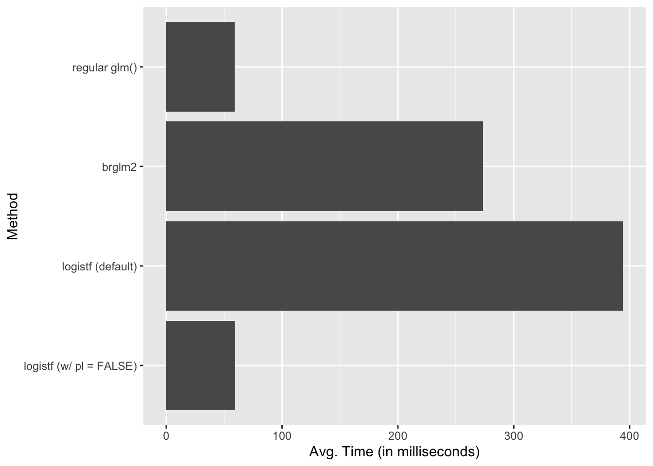
In short, logistf is slower than brglm2, but only because it computes the profile likelihood p-values by default. Once we skip those calculations using pl = FALSE, logistf is much faster, roughly as fast as glm() itself.

Here’s a plot showing the computation times of the four fits. Remember that all of these are computed practically instantly, so it only makes a difference when the fits are done thousands of times, like in a Monte Carlo simulation.

# plot times
bm %>%
  group_by(expr) %>%
  summarize(avg_time = mean(time)*1e-6) %>%  # convert to milliseconds
  ggplot(aes(x = fct_rev(expr), y = avg_time)) + 
  geom_col() + 
  labs(x = "Method", 
       y = "Avg. Time (in milliseconds)") + 
  coord_flip()

Follow-Up Notes

The models return slightly different estimates. Maybe they are using slightly different convergence tolerances. I didn’t investigate this beyond noticing it.

cbind(coef(f2()), coef(f4()))

                  [,1]       [,2]
(Intercept) -0.4771934 -0.4771935
polity_conq -2.2771109 -2.2771117
lndist       3.4020239  3.4020215
terrain      1.1018697  1.1018713
soldperterr -0.5952096 -0.5952110
gdppc2      -1.1542009 -1.1541998
coord        3.0514480  3.0514473

Ioannis Kosmidis made me aware of two things.

1. logistf has a C backend (thus explaining the speed).
2. brglm2’s fitting routine for logistic regression is written entirely in R. (brglm2 is also more general; it supports a variety of models and corrections).

Computer

Here’s the info on my machine.

system("sysctl -n machdep.cpu.brand_string", intern = TRUE)

[1] "Apple M2 Max"

References

Firth, David. 1993. “Bias Reduction of Maximum Likelihood Estimates.” Biometrika 80 (1): 27–38. https://doi.org/10.1093/biomet/80.1.27.

Kosmidis, Ioannis, and David Firth. 2021. “Jeffreys-Prior Penalty, Finiteness and Shrinkage in Binomial-Response Generalized Linear Models.” Biometrika 108 (1): 71–82. https://doi.org/10.1093/biomet/asaa052.

Rainey, Carlisle, and Kelly McCaskey. 2021. “Estimating Logit Models with Small Samples.” Political Science Research and Methods 9 (3): 549–64. https://doi.org/10.1017/psrm.2021.9.

Weisiger, Alex. 2014. “Victory Without Peace: Conquest, Insurgency, and War Termination.” Conflict Management and Peace Science 31 (4): 357–82. https://doi.org/10.1177/0738894213508691.