Example: Law of Coercive Responsiveness

In this example, we download Fariss’ human rights score data set, download the dissent score data set, and plot the correlation between the two.

Orienting this correlation theoretically, we quote Davenport (2007) on “The Law of Coercive Responsiveness:”

By far the most long-standing and stable influence on state repression concerns political conflict. Dating back to, at least, Kautilya in India during the fourth century (particularly Book IV in the Arthashastra) or, more familiar to those in the West, Niccolo Machiavelli in Italy during the late 1400s and early 1500s or Thomas Hobbes in England during the late 1500s and early 1600s, it has been commonly thought that governing authorities should respond with repression to behavior that threatens the political system, government personnel, the economy, or the lives, beliefs, and livelihoods of those within their territorial jurisdiction. Quiescence is a major benefit to political authorities, supporting the extraction of taxes, the creation of wealth, and a major part of their legitimacy as a protector. Considering different time periods and countries, as well as a wide variety of measurements for both conflict and repression, every statistical investigation of the subject has found a positive influence. When challenges to the status quo take place, authorities generally employ some form of repressive action to counter or eliminate the behavioral threat; in short, there appears to be a “Law of Coercive Responsiveness.”

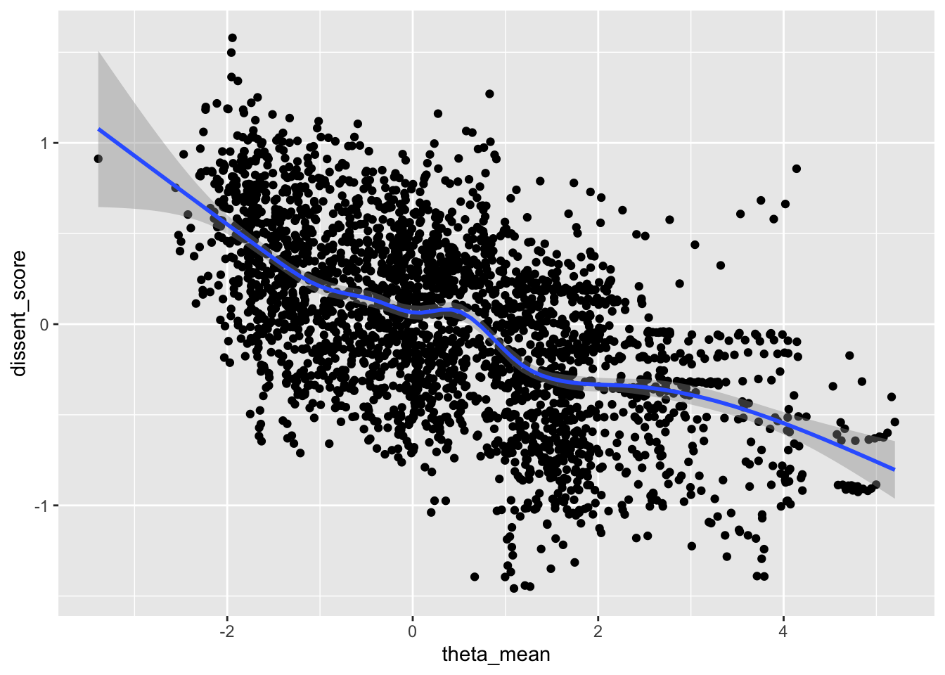
In brief, Davenport points out the correlation between the level of repression and the level of dissent. As an example, we show that correlation using our dissent score and Fariss’ human rights protection score.

# load packages
library(tidyverse)
library(dataverse)

# download latest version V4.01 of fariss' human rights protection scores
hrp_scores <- get_dataframe_by_name(
  filename = "HumanRightsProtectionScores_v4.01.tab",
  dataset = "10.7910/DVN/RQ85GK",
  server = "dataverse.harvard.edu") |>
  # change variable names to match those used in the dissent scores
  select(year = YEAR, ccode = COW, theta_mean) |>
  glimpse()
Rows: 11,275
Columns: 3
$ year       <dbl> 1946, 1947, 1948, 1949, 1950, 1951, 1952, 1953, 1954, 1955,…
$ ccode      <dbl> 2, 2, 2, 2, 2, 2, 2, 2, 2, 2, 2, 2, 2, 2, 2, 2, 2, 2, 2, 2,…
$ theta_mean <dbl> -0.7830982, -0.8748142, -0.9997263, -1.1701207, -1.2525558,…
# download latest version of dissent score data set
dissent <- get_dataframe_by_name(
  filename = "dissent-scores.tab",
  dataset  = "doi:10.7910/DVN/CL4CA8",
  server   = "dataverse.harvard.edu", 
  original = TRUE, 
  .f = readr::read_csv) |>
  glimpse()
Rows: 2,775
Columns: 15
$ release             <chr> "V0.1 (Preprint)", "V0.1 (Preprint)", "V0.1 (Prepr…
$ release_date        <date> 2023-12-18, 2023-12-18, 2023-12-18, 2023-12-18, 2…
$ data_source         <chr> "IDEA", "IDEA", "IDEA", "IDEA", "IDEA", "IDEA", "I…
$ created_date        <date> 2023-12-18, 2023-12-18, 2023-12-18, 2023-12-18, 2…
$ country_name        <chr> "United States", "United States", "United States",…
$ ccode               <dbl> 2, 2, 2, 2, 2, 2, 2, 2, 2, 2, 2, 2, 2, 2, 2, 20, 2…
$ stateabb            <chr> "USA", "USA", "USA", "USA", "USA", "USA", "USA", "…
$ year                <dbl> 1990, 1991, 1992, 1993, 1994, 1995, 1996, 1997, 19…
$ n_events            <dbl> 135537, 140735, 151180, 177717, 194368, 195981, 20…
$ n_dissent_events    <dbl> 118, 109, 124, 138, 127, 117, 123, 130, 147, 121, …
$ frac_dissent_events <dbl> 0.0008706110, 0.0007745053, 0.0008202143, 0.000776…
$ avg_pi              <dbl> 0.0008690543, 0.0007750752, 0.0008211722, 0.000779…
$ avg_eta             <dbl> -7.051493, -7.166315, -7.107983, -7.160229, -7.331…
$ dissent_score       <dbl> -0.62807636, -0.67911036, -0.65318394, -0.67640508…
$ se_dissent_score    <dbl> 0.04107096, 0.04241524, 0.03997557, 0.03736980, 0.…
# join the two by ccode and year
joined <- left_join(dissent, hrp_scores) |>
  glimpse()
Rows: 2,775
Columns: 16
$ release             <chr> "V0.1 (Preprint)", "V0.1 (Preprint)", "V0.1 (Prepr…
$ release_date        <date> 2023-12-18, 2023-12-18, 2023-12-18, 2023-12-18, 2…
$ data_source         <chr> "IDEA", "IDEA", "IDEA", "IDEA", "IDEA", "IDEA", "I…
$ created_date        <date> 2023-12-18, 2023-12-18, 2023-12-18, 2023-12-18, 2…
$ country_name        <chr> "United States", "United States", "United States",…
$ ccode               <dbl> 2, 2, 2, 2, 2, 2, 2, 2, 2, 2, 2, 2, 2, 2, 2, 20, 2…
$ stateabb            <chr> "USA", "USA", "USA", "USA", "USA", "USA", "USA", "…
$ year                <dbl> 1990, 1991, 1992, 1993, 1994, 1995, 1996, 1997, 19…
$ n_events            <dbl> 135537, 140735, 151180, 177717, 194368, 195981, 20…
$ n_dissent_events    <dbl> 118, 109, 124, 138, 127, 117, 123, 130, 147, 121, …
$ frac_dissent_events <dbl> 0.0008706110, 0.0007745053, 0.0008202143, 0.000776…
$ avg_pi              <dbl> 0.0008690543, 0.0007750752, 0.0008211722, 0.000779…
$ avg_eta             <dbl> -7.051493, -7.166315, -7.107983, -7.160229, -7.331…
$ dissent_score       <dbl> -0.62807636, -0.67911036, -0.65318394, -0.67640508…
$ se_dissent_score    <dbl> 0.04107096, 0.04241524, 0.03997557, 0.03736980, 0.…
$ theta_mean          <dbl> 1.5452468, 1.3345563, 1.2958548, 1.4114671, 1.4772…
# plot the relationship between theta_mean and the dissent score
ggplot(joined, aes(x = theta_mean, y = dissent_score)) + 
  geom_point() + 
  geom_smooth()